Capsule Networks: A Quick Primer

Whether you're new to deep learning or a serious researcher, you've surely encountered the term Convolutional Neural Networks. They are one of the most researched and top-performing architectures in the field. That being said, CNNs have a few drawbacks in recognizing features of input data when they are in different orientations. To address this problem, Geoffrey E. Hinton, together with his team Sara Sabour and Nicholas Frosst, came up with a new type of Neural Network. They called them Capsule Networks.

In this article we’ll discuss the following topics to give an introduction to capsule networks:

• Convolutional Neural Networks and the Orientation Problem
• Problems with Pooling in CNNs
• Intuition Behind Capsule Networks
• Capsule Networks Architecture
• Final Notes

Convolutional Neural Networks and the Orientation Problem

Convolutional neural networks are one of the most popular deep learning architectures that are widely used for computer vision applications. From image classification to object detection and segmentation, CNNs have defined state of the art results. That being said, these networks have their own complications and difficulties for different types of images. Let's start with their origins, then see how they're currently performing.

Yann LeCun first proposed the CNN in the year 1998. He was then able to detect handwritten digits with a simple five-layer convolutional neural network that was trained on the MNIST dataset, containing over 60,000 examples. The idea is simple: train the network, identify the features in the images, and classify them. Then in 2019, EfficientNet-B7 achieved the state of the art performance in classifying images on the ImageNet Dataset. The network can identify the label of a particular picture from over 1.2 million images with 84.4% of accuracy.

Looking at these results and progress, we can infer that convolutional approaches make it possible to learn many sophisticated features with simple computations. By performing many matrix multiplications and summations on our input, we can arrive at a reliable answer to our question.

But CNNs are not perfect. If CNNs are fed with images of different sizes and orientations, they fail.

Let me run through an example. Say you rotate a face upside down and then feed it to a CNN; it would not be able to identify features like the eyes, nose, or mouth. Similarly, if you reconstruct specific regions of the face (i.e., switch the positions of the nose and eyes), the network will still be able to recognize the face—even though it isn't exactly a face anymore. In short, CNNs can learn the patterns of the images statistically, but not what the actual image looks like in different orientations.

The Problem with Pooling in CNNs

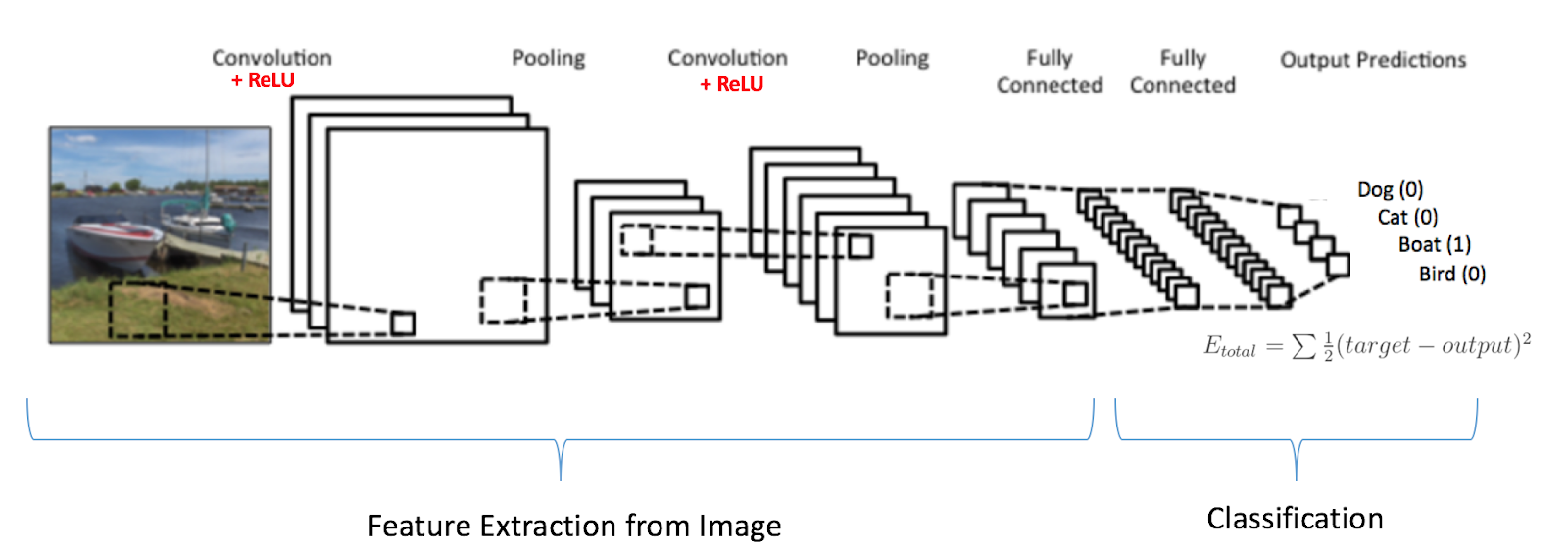
To understand pooling, one must know how a CNN works. The building block of CNNs is the convolutional layer. These layers are responsible for identifying the features in a given image, like the curves, edges, sharpness, and color. In the end, the fully connected layers of the network will combine very high-level features and produce classification predictions. You can see below what a basic convolutional network looks like.

The authors use the max/average pooling operation, or have successive convolutional layers throughout the network. The pooling operation reduces unnecessary information. Using this design, we can reduce the spacial size of the data flowing through the network, and thus increase the "field of view" of the neurons in higher layers, allowing them to detect higher-order features in a broader region of the input image. This is how max-pooling operations in CNNs help achieve state of the art performance. That being said, we should not be fooled by its performance; CNNs work better than any model before them, but max-pooling is nevertheless losing valuable information.

Geoffrey Hinton stated in one of his lectures:

"The pooling operation used in convolutional neural networks is a big mistake, and the fact that it works so well is a disaster!"

Now let’s see how Capsule Networks overcome this problem.

How Capsule Networks Work

To overcome this problem involving the rotational relationships in images, Hinton and Sabour drew inspiration from neuroscience. They explain that the brain is organized into modules, which can be considered capsules. With this in mind, they proposed capsule networks which incorporate dynamic routing algorithms to estimate features of objects like pose (position, size, orientation, deformation, velocity, albedo, hue, texture, and so on). This research was published in 2017, in their paper titled Dynamic Routing Between Capsules.

So, what are "capsules"? And how does dynamic routing work?

What Are Capsules in a Capsule Network?

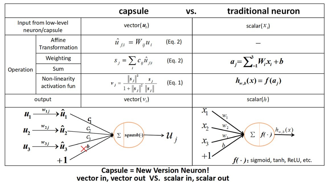
Unlike normal neurons, capsules perform their computations on their inputs and then "encapsulate" the results into a small vector of highly informative outputs. A capsule could be considered a replacement or substitute for your average artificial neuron; whereas an artificial neuron deals with scalars, a capsule deals with vectors. For instance, we could summarize the steps taken by an artificial neuron as follows:

1. Multiply the input scalars with the weighted connections between the neurons.
2. Compute the weighted sum of the input scalars.
3. Apply an activation function (scalar nonlinearity) to get the output.

A capsule, on the other hand, goes through several steps in addition to those listed above, in order to achieve the affine transformation (preserving co-linearity and ratio of distances) of the input. Here, the process is as follows:

1. Multiply the input vectors by the weight matrices (which encode spatial relationships between low-level features and high-level features) (matrix multiplication).
2. Multiply the result by the weights.
3. Compute the weighted sum of the input vectors.
4. Apply an activation function (vector non-linearity) to get the output.

Let's take a more detailed look at each step to better understand how a capsule works.

1. Multiply the input vectors by the weight matrices (affine transformation)

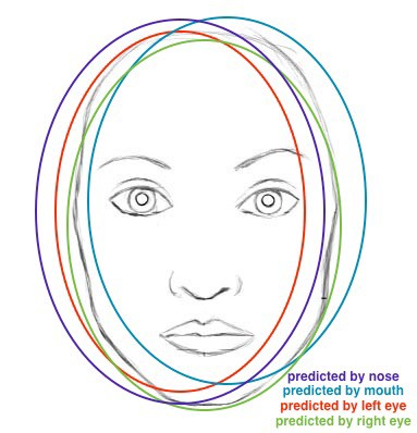
The input vectors represent either the initial input, or an input provided by an earlier layer in the network. These vectors are first multiplied by the weight matrices. The weight matrix, as described previously, captures the spatial relationships. Say that one object is centered around another, and they are equally proportioned in size. The product of the input vector and the weight matrix will signify the high-level feature. For example, if the low-level features are nose, mouth, left eye, and right eye, then if the predictions of the four low-level features point to the same orientation and state of a face, a face will be what's predicted (as shown below). This is what the "high-level" feature is.

2. Multiply the result by the weights

In this step, the outputs obtained from the previous step are multiplied by the weights of the network. What can the weights be? In a usual artificial neural network (ANN), the weights are adjusted based on the error rate, followed by backpropagation. However, this mechanism isn’t applied in a Capsule Network. Dynamic routing is what determines the modification of weights in a network. This defines the strategy for assigning weights to the neurons' connections.

A capsule network adjusts the weights such that a low-level capsule is strongly associated with high-level capsules that are in its proximity. The proximity measure is determined by the affine transformation step we discussed previously (Step 1). The distance between the outputs obtained from the affine transformation step and the dense clusters of the predictions of low-level capsules is computed (the dense clusters could be formed if the predictions made by the low-level capsules are similar, thus lying near to each other). The high-level capsule that has the minimum distance between the cluster of already made predictions and the newly predicted one will have a higher weight, and the remaining capsules would be assigned lower weights, based on the distance metric.

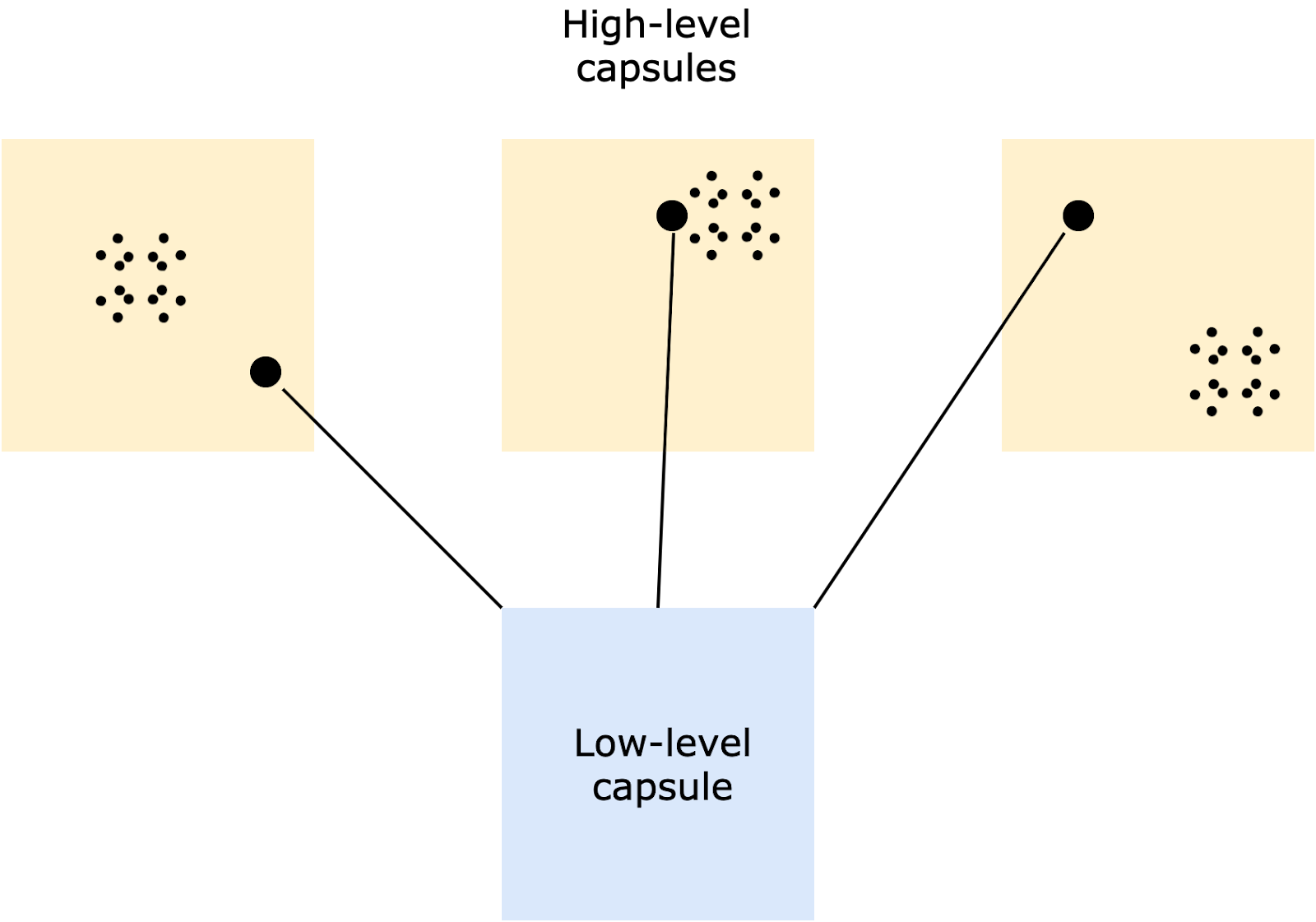
In the above image, the weights would be assigned in the following order: middle > left > right. In a nutshell, the essence of the dynamic routing algorithm could be seen as this: the lower level capsule will send its input to the higher level capsule that “agrees” with its input.

3. Compute the weighted sum of the input vectors

This sums up all the outputs obtained from the previous step.

4. Apply an activation function (vector non-linearity) to get the output

In a capsule network, the vector non-linearity is obtained by "squashing" (i.e. via an activation function) the output vector, for it to have a length of 1 and a constant direction. The non-linearity function is given by:

Where s_j is the output obtained from the previous step, and v_j is the output obtained after applying the non-linearity. The left side of the equation performs additional squashing, while the right side of the equation performs unit scaling of the output vector.

On the whole, the dynamic routing algorithm is thus summarized:

Line 1: This line defines the procedure of ROUTING, which takes affine transformed input (u), the number of routing iterations (r), and the layer number (l) as inputs.

Line 2: b_ij is a temporary value that is used to initialize c_i in the end.

Line 3: The for loop iterates ‘r’ times.

Line 4: The softmax function applied to b_i makes sure to output a non-negative c_i, where all the outputs sum to 1.

Line 5: For every capsule in the succeeding layer, the weighted sum is computed.

Line 6: For every capsule in the succeeding layer, the weighted sum is squashed.

Line 7: The weights b_ij are updated here. u_ji denotes the input to the capsule from low-level capsule i, and v_j denotes the output of high-level capsule j.

CapsNet Architecture

The CapsNet architecture consists of an encoder and a decoder, where each has a set of three layers. An encoder has a convolutional layer, PrimaryCaps layer, and a DigitCaps layer; the decoder has 3 fully-connected layers.

Let's now look into each of these networks. We'll consider this in context of the MNIST dataset, for example.

Encoder Network

An encoder has two convolutional layers and one fully-connected layer. The first convolutional layer, Conv1, has 256 9×9 convolutional kernels with a stride of 1, and a ReLU activation function. This layer is responsible for converting the pixel intensities to the activities of local feature detectors, which are then fed to the PrimaryCaps layer. The PrimaryCaps layer is a convolutional layer that has 32 channels of convolutional 8-D capsules (each capsule has 8 convolutional units with a 9×9 kernel and a stride of 2). Primary capsules perform inverse graphics, meaning they reverse-engineer the process of the actual image generation. The capsule applies eight 9×9×256 kernels onto the 20×20×256 input volume, which gives a 6×6×8 output tensor. As there are 32 8-D capsules, the output would thus be of size 6×6×8×32. The DigitCaps layer has 16-D capsules per class, where each capsule receives input from the low-level capsule.

The 8×16 W_ij is the weight matrix used for affine transformation against each 8-D capsule. The routing mechanism discussed previously always exists between two capsule layers (say, between PrimaryCaps and DigitCaps).

In the end, a reconstruction loss is used to encode the instantiation parameters. The loss is calculated for each training example against all the output classes. The total loss is the sum of losses of all the digit capsules. The loss equation is given by:

Where:

T_k = 1 if a digit of class k is present

m⁺ = 0.9

m^- = 0.1

v_k = vector obtained from DigitCaps layer

The first term of the equation represents the loss for a correct DigitCaps, and the second term represents the loss for an incorrect DigitCaps.

Decoder Network

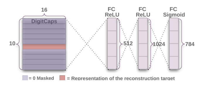
A decoder takes the correct 16-D digit capsule and decodes it into an image. None of the incorrect digit capsules are taken into consideration. The loss is calculated by finding the Euclidean distance between the input image and the reconstructed image.

A decoder has three fully-connected layers. The first layer has 512 neurons; the second has 1024 neurons; and the third has 784 neurons (giving 28×28 reconstructed images for MNIST).

Final Notes

A Capsule Network could be considered a "real-imitation" of the human brain. Unlike convolutional neural networks, which do not evaluate the spatial relationships in the given data, capsule networks consider the orientation of parts in an image as a key part of data analysis. They examine these hierarchical relationships to better identify images. The inverse-graphics mechanism which our brains make use of is imitated here to build a hierarchical representation of an image, and match it with what the network has learned. Though it isn’t yet computationally efficient, there does seem to be an accuracy boost beneficial in tackling real-world scenarios. The Dynamic Routing of Capsules is what makes all of this possible. It employs an unusual strategy of updating the weights in a network, thus avoiding the pooling operation. As time passes by, capsule networks will surely penetrate into various other fields, making machines even more human-like.