How to Train YOLO v5 on a Custom Dataset

Oct. 20, 2022 update - this tutorial now features some deprecated code for sourcing the dataset. Please, see our updated tutorial on YOLOv7 for additional instructions on getting the dataset in a Gradient Notebook for this demo.

YOLO, or You Only Look Once, is one of the most widely used deep learning based object detection algorithms out there. In this tutorial, we will go over how to train one of its latest variants, YOLOv5, on a custom dataset. More precisely, we will train the YOLO v5 detector on a road sign dataset. By the end of this post, you shall have yourself an object detector that can localize and classify road signs.

You can also run this code on a free GPU using the Gradient Notebook for this post.

Before we begin, let me acknowledge that YOLOv5 attracted quite a bit of controversy when it was released over whether it's right to call it v5. I've addressed this a bit at the end of this article. For now, I'd simply say that I'm referring to the algorithm as YOLOv5 since it is what the name of the code repository is.

My decision to go with YOLOv5 over other variants is due to the fact that it's the most actively maintained Python port of YOLO. Other variants like YOLO v4 are written in C, which might not be as accessible to the typical deep learning practitioner as Python.

With that said, let's get started.

This post is structured as follows.

• Set up the Code
• Download the Data
• Convert the Annotations into the YOLO v5 Format
  • YOLO v5 Annotation Format
  • Testing the annotations
  • Partition the Dataset
• Training Options
  • Data Config File
  • Hyper-parameter Config File
  • Custom Network Architecture
  • Train the Model
• Inference
  • Computing the mAP on test dataset
• Conclusion... and a bit about the naming saga

Set up the code

We begin by cloning the YOLO v5 repository and setting up the dependencies required to run YOLO v5. You might need sudo rights to install some of the packages.

In a terminal, type:

git clone https://github.com/ultralytics/yolov5

I recommend you create a new conda or a virtualenv environment to run your YOLO v5 experiments as to not mess up dependencies of any existing project.

Once you have activated the new environment, install the dependencies using pip. Make sure that the pip you are using is that of the new environment. You can do so by typing in terminal.

which pip

For me, it shows something like this.

/home/ayoosh/miniconda3/envs/yolov5/bin/pip

It tells me that the pip I'm using is of the new environment called yolov5 that I just created. If you are using a pip belonging to a different environment, your python would be installed to that different library and not to the one you created.

With that sorted, let us go ahead with the installation.

pip install -r yolov5/requirements.txt

With the dependencies installed, let us now import the required modules to conclude setting up the code.

import torch
from IPython.display import Image  # for displaying images
import os 
import random
import shutil
from sklearn.model_selection import train_test_split
import xml.etree.ElementTree as ET
from xml.dom import minidom
from tqdm import tqdm
from PIL import Image, ImageDraw
import numpy as np
import matplotlib.pyplot as plt

random.seed(108)

Download the Data

For this tutorial, we are going to use an object detection dataset of road signs from MakeML.

It is a dataset that contains road signs belonging to 4 classes:

1. Traffic Light
2. Stop
3. Speed Limit
4. Crosswalk

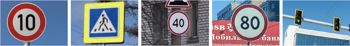
The dataset is a small one, containing only 877 images in total. While you may want to train with a larger dataset (like the LISA Dataset) to fully realize the capabilities of YOLO, we use a small dataset in this tutorial to facilitate quick prototyping. Typical training takes less than half an hour and this would allow you to quickly iterate with experiments involving different hyperparamters.

We create a directory called Road_Sign_Dataset to keep our dataset now. This directory needs to be in the same folder as the yolov5 repository folder we just cloned.

mkdir Road_Sign_Dataset
cd Road_Sign_Dataset

Download the dataset.

wget -O RoadSignDetectionDataset.zip https://arcraftimages.s3-accelerate.amazonaws.com/Datasets/RoadSigns/RoadSignsPascalVOC.zip?region=us-east-2

Unzip the dataset.

unzip RoadSignDetectionDataset.zip

Delete the unneeded files.

rm -r __MACOSX RoadSignDetectionDataset.zip

Convert the Annotations into the YOLO v5 Format

In this part, we convert annotations into the format expected by YOLO v5. There are a variety of formats when it comes to annotations for object detection datasets.

Annotations for the dataset we downloaded follow the PASCAL VOC XML format, which is a very popular format. Since this a popular format, you can find online conversion tools. Nevertheless, we are going to write the code for it to give you some idea of how to convert lesser popular formats as well (for which you may not find popular tools).

The PASCAL VOC format stores its annotation in XML files where various attributes are described by tags. Let us look at one such annotation file.

# Assuming you're in the data folder
cat annotations/road4.xml

The output looks like the following.

<annotation>
    <folder>images</folder>
    <filename>road4.png</filename>
    <size>
        <width>267</width>
        <height>400</height>
        <depth>3</depth>
    </size>
    <segmented>0</segmented>
    <object>
        <name>trafficlight</name>
        <pose>Unspecified</pose>
        <truncated>0</truncated>
        <occluded>0</occluded>
        <difficult>0</difficult>
        <bndbox>
            <xmin>20</xmin>
            <ymin>109</ymin>
            <xmax>81</xmax>
            <ymax>237</ymax>
        </bndbox>
    </object>
    <object>
        <name>trafficlight</name>
        <pose>Unspecified</pose>
        <truncated>0</truncated>
        <occluded>0</occluded>
        <difficult>0</difficult>
        <bndbox>
            <xmin>116</xmin>
            <ymin>162</ymin>
            <xmax>163</xmax>
            <ymax>272</ymax>
        </bndbox>
    </object>
    <object>
        <name>trafficlight</name>
        <pose>Unspecified</pose>
        <truncated>0</truncated>
        <occluded>0</occluded>
        <difficult>0</difficult>
        <bndbox>
            <xmin>189</xmin>
            <ymin>189</ymin>
            <xmax>233</xmax>
            <ymax>295</ymax>
        </bndbox>
    </object>
</annotation>

The above annotation file describes a file named road4.jpg that has a dimensions of 267 x 400 x 3. It has 3 object tags which represent 3 bounding boxes. The class is specified by the name tag, whereas the details of the bounding box are represented by the bndbox tag. A bounding box is described by the coordinates of its top-left (x_min, y_min) corner and its bottom-right (xmax, ymax) corner.

YOLO v5 Annotation Format

YOLO v5 expects annotations for each image in form of a .txt file where each line of the text file describes a bounding box. Consider the following image.

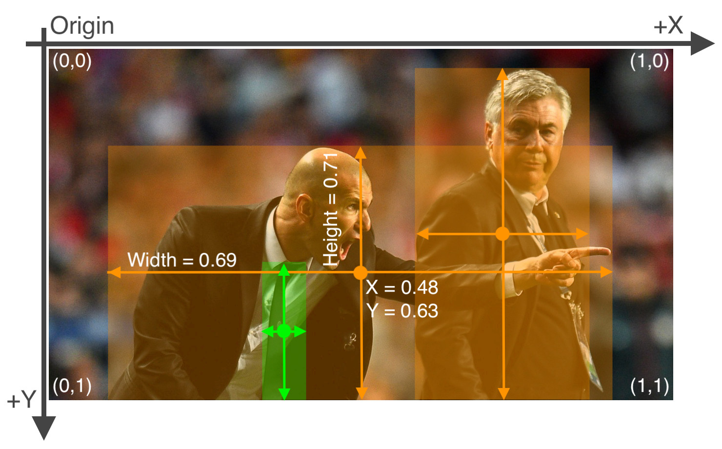
The annotation file for the image above looks like the following:

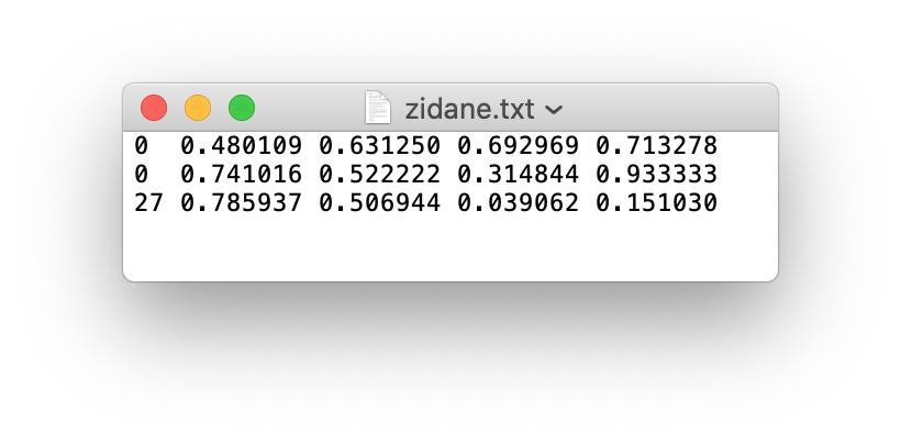
There are 3 objects in total (2 persons and one tie). Each line represents one of these objects. The specification for each line is as follows.

• One row per object
• Each row is class x_center y_center width height format.
• Box coordinates must be normalized by the dimensions of the image (i.e. have values between 0 and 1)
• Class numbers are zero-indexed (start from 0).

We now write a function that will take the annotations in VOC format and convert them to a format where information about the bounding boxes are stored in a dictionary.

# Function to get the data from XML Annotation
def extract_info_from_xml(xml_file):
    root = ET.parse(xml_file).getroot()
    
    # Initialise the info dict 
    info_dict = {}
    info_dict['bboxes'] = []

    # Parse the XML Tree
    for elem in root:
        # Get the file name 
        if elem.tag == "filename":
            info_dict['filename'] = elem.text
            
        # Get the image size
        elif elem.tag == "size":
            image_size = []
            for subelem in elem:
                image_size.append(int(subelem.text))
            
            info_dict['image_size'] = tuple(image_size)
        
        # Get details of the bounding box 
        elif elem.tag == "object":
            bbox = {}
            for subelem in elem:
                if subelem.tag == "name":
                    bbox["class"] = subelem.text
                    
                elif subelem.tag == "bndbox":
                    for subsubelem in subelem:
                        bbox[subsubelem.tag] = int(subsubelem.text)            
            info_dict['bboxes'].append(bbox)
    
    return info_dict

Let us try this function on an annotation file.

print(extract_info_from_xml('annotations/road4.xml'))

This outputs:

{'bboxes': [{'class': 'trafficlight', 'xmin': 20, 'ymin': 109, 'xmax': 81, 'ymax': 237}, {'class': 'trafficlight', 'xmin': 116, 'ymin': 162, 'xmax': 163, 'ymax': 272}, {'class': 'trafficlight', 'xmin': 189, 'ymin': 189, 'xmax': 233, 'ymax': 295}], 'filename': 'road4.png', 'image_size': (267, 400, 3)}

We now write a function to convert information contained in info_dict to YOLO v5 style annotations and write them to a txt file. In case your annotations are different than PASCAL VOC ones, you can write a function to convert them to the info_dict format and use the function below to convert them to YOLO v5 style annotations.

# Dictionary that maps class names to IDs
class_name_to_id_mapping = {"trafficlight": 0,
                           "stop": 1,
                           "speedlimit": 2,
                           "crosswalk": 3}

# Convert the info dict to the required yolo format and write it to disk
def convert_to_yolov5(info_dict):
    print_buffer = []
    
    # For each bounding box
    for b in info_dict["bboxes"]:
        try:
            class_id = class_name_to_id_mapping[b["class"]]
        except KeyError:
            print("Invalid Class. Must be one from ", class_name_to_id_mapping.keys())
        
        # Transform the bbox co-ordinates as per the format required by YOLO v5
        b_center_x = (b["xmin"] + b["xmax"]) / 2 
        b_center_y = (b["ymin"] + b["ymax"]) / 2
        b_width    = (b["xmax"] - b["xmin"])
        b_height   = (b["ymax"] - b["ymin"])
        
        # Normalise the co-ordinates by the dimensions of the image
        image_w, image_h, image_c = info_dict["image_size"]  
        b_center_x /= image_w 
        b_center_y /= image_h 
        b_width    /= image_w 
        b_height   /= image_h 
        
        #Write the bbox details to the file 
        print_buffer.append("{} {:.3f} {:.3f} {:.3f} {:.3f}".format(class_id, b_center_x, b_center_y, b_width, b_height))
        
    # Name of the file which we have to save 
    save_file_name = os.path.join("annotations", info_dict["filename"].replace("png", "txt"))
    
    # Save the annotation to disk
    print("\n".join(print_buffer), file= open(save_file_name, "w"))

Now we convert all the xml annotations into YOLO style txt ones.

# Get the annotations
annotations = [os.path.join('annotations', x) for x in os.listdir('annotations') if x[-3:] == "xml"]
annotations.sort()

# Convert and save the annotations
for ann in tqdm(annotations):
    info_dict = extract_info_from_xml(ann)
    convert_to_yolov5(info_dict)
annotations = [os.path.join('annotations', x) for x in os.listdir('annotations') if x[-3:] == "txt"]

Testing the annotations

Just for a sanity check, let us now test some of these transformed annotations. We randomly load one of the annotations and plot boxes using the transformed annotations, and visually inspect it to see whether our code has worked as intended.

Run the next cell multiple times. Every time, a random annotation is sampled.

random.seed(0)

class_id_to_name_mapping = dict(zip(class_name_to_id_mapping.values(), class_name_to_id_mapping.keys()))

def plot_bounding_box(image, annotation_list):
    annotations = np.array(annotation_list)
    w, h = image.size
    
    plotted_image = ImageDraw.Draw(image)

    transformed_annotations = np.copy(annotations)
    transformed_annotations[:,[1,3]] = annotations[:,[1,3]] * w
    transformed_annotations[:,[2,4]] = annotations[:,[2,4]] * h 
    
    transformed_annotations[:,1] = transformed_annotations[:,1] - (transformed_annotations[:,3] / 2)
    transformed_annotations[:,2] = transformed_annotations[:,2] - (transformed_annotations[:,4] / 2)
    transformed_annotations[:,3] = transformed_annotations[:,1] + transformed_annotations[:,3]
    transformed_annotations[:,4] = transformed_annotations[:,2] + transformed_annotations[:,4]
    
    for ann in transformed_annotations:
        obj_cls, x0, y0, x1, y1 = ann
        plotted_image.rectangle(((x0,y0), (x1,y1)))
        
        plotted_image.text((x0, y0 - 10), class_id_to_name_mapping[(int(obj_cls))])
    
    plt.imshow(np.array(image))
    plt.show()

# Get any random annotation file 
annotation_file = random.choice(annotations)
with open(annotation_file, "r") as file:
    annotation_list = file.read().split("\n")[:-1]
    annotation_list = [x.split(" ") for x in annotation_list]
    annotation_list = [[float(y) for y in x ] for x in annotation_list]

#Get the corresponding image file
image_file = annotation_file.replace("annotations", "images").replace("txt", "png")
assert os.path.exists(image_file)

#Load the image
image = Image.open(image_file)

#Plot the Bounding Box
plot_bounding_box(image, annotation_list)

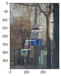
Great, we are able to recover the correct annotation from the YOLO v5 format. This means we have implemented the conversion function properly.

Partition the Dataset

Next we partition the dataset into train, validation, and test sets containing 80%, 10%, and 10% of the data, respectively. You can change the split values according to your convenience.

# Read images and annotations
images = [os.path.join('images', x) for x in os.listdir('images')]
annotations = [os.path.join('annotations', x) for x in os.listdir('annotations') if x[-3:] == "txt"]

images.sort()
annotations.sort()

# Split the dataset into train-valid-test splits 
train_images, val_images, train_annotations, val_annotations = train_test_split(images, annotations, test_size = 0.2, random_state = 1)
val_images, test_images, val_annotations, test_annotations = train_test_split(val_images, val_annotations, test_size = 0.5, random_state = 1)

Create the folders to keep the splits.

!mkdir images/train images/val images/test annotations/train annotations/val annotations/test

Move the files to their respective folders.

#Utility function to move images 
def move_files_to_folder(list_of_files, destination_folder):
    for f in list_of_files:
        try:
            shutil.move(f, destination_folder)
        except:
            print(f)
            assert False

# Move the splits into their folders
move_files_to_folder(train_images, 'images/train')
move_files_to_folder(val_images, 'images/val/')
move_files_to_folder(test_images, 'images/test/')
move_files_to_folder(train_annotations, 'annotations/train/')
move_files_to_folder(val_annotations, 'annotations/val/')
move_files_to_folder(test_annotations, 'annotations/test/')

Rename the annotations folder to labels, as this is where YOLO v5 expects the annotations to be located in.

mv annotations labels
cd ../yolov5 

Training Options

Now, we train the network. We use various flags to set options regarding training.

• img        : Size of image. The image is a square one. The original image is resized while maintaining the aspect ratio. The longer side of the image is resized to this number. The shorter side is padded with grey color.

• batch: The batch size
• epochs: Number of epochs to train for
• data: Data YAML file that contains information about the dataset (path of images, labels)
• workers: Number of CPU workers
• cfg: Model architecture. There are 4 choices available: yolo5s.yaml, yolov5m.yaml, yolov5l.yaml, yolov5x.yaml. The size and complexity of these models increases in the ascending order and you can choose a model which suits the complexity of your object detection task. In case you want to work with a custom architecture, you will have to define a YAML file in the models folder specifying the network architecture.
• weights: Pretrained weights you want to start training from. If you want to train from scratch, use --weights ' '
• name: Various things about training such as train logs. Training weights would be stored in a folder named runs/train/name
• hyp: YAML file that describes hyperparameter choices. For examples of how to define hyperparameters, see data/hyp.scratch.yaml. If unspecified, the file data/hyp.scratch.yaml is used.

Data Config File

Details for the dataset you want to train your model on are defined by the data config YAML file. The following parameters have to be defined in a data config file:

1. train, test, and val: Locations of train, test, and validation images.
2. nc: Number of classes in the dataset.
3. names: Names of the classes in the dataset. The index of the classes in this list would be used as an identifier for the class names in the code.

Create a new file called road_sign_data.yaml and place it in the yolov5/data folder. Then populate it with the following.

train: ../Road_Sign_Dataset/images/train/ 
val:  ../Road_Sign_Dataset/images/val/
test: ../Road_Sign_Dataset/images/test/

# number of classes
nc: 4

# class names
names: ["trafficlight","stop", "speedlimit","crosswalk"]

YOLO v5 expects to find the training labels for the images in the folder whose name can be derived by replacing images with labels in the path to dataset images. For example, in the example above, YOLO v5 will look for train labels in ../Road_Sign_Dataset/labels/train/.

Or you can simply download the file.

!wget -P data/ https://gist.githubusercontent.com/ayooshkathuria/bcf7e3c929cbad445439c506dba6198d/raw/f437350c0c17c4eaa1e8657a5cb836e65d8aa08a/road_sign_data.yaml

Hyperparameter Config File

The hyperparameter config file helps us define the hyperparameters for our neural network. We are going to use the default one, data/hyp.scratch.yaml. This is what it looks like.

# Hyperparameters for COCO training from scratch
# python train.py --batch 40 --cfg yolov5m.yaml --weights '' --data coco.yaml --img 640 --epochs 300
# See tutorials for hyperparameter evolution https://github.com/ultralytics/yolov5#tutorials


lr0: 0.01  # initial learning rate (SGD=1E-2, Adam=1E-3)
lrf: 0.2  # final OneCycleLR learning rate (lr0 * lrf)
momentum: 0.937  # SGD momentum/Adam beta1
weight_decay: 0.0005  # optimizer weight decay 5e-4
warmup_epochs: 3.0  # warmup epochs (fractions ok)
warmup_momentum: 0.8  # warmup initial momentum
warmup_bias_lr: 0.1  # warmup initial bias lr
box: 0.05  # box loss gain
cls: 0.5  # cls loss gain
cls_pw: 1.0  # cls BCELoss positive_weight
obj: 1.0  # obj loss gain (scale with pixels)
obj_pw: 1.0  # obj BCELoss positive_weight
iou_t: 0.20  # IoU training threshold
anchor_t: 4.0  # anchor-multiple threshold
# anchors: 3  # anchors per output layer (0 to ignore)
fl_gamma: 0.0  # focal loss gamma (efficientDet default gamma=1.5)
hsv_h: 0.015  # image HSV-Hue augmentation (fraction)
hsv_s: 0.7  # image HSV-Saturation augmentation (fraction)
hsv_v: 0.4  # image HSV-Value augmentation (fraction)
degrees: 0.0  # image rotation (+/- deg)
translate: 0.1  # image translation (+/- fraction)
scale: 0.5  # image scale (+/- gain)
shear: 0.0  # image shear (+/- deg)
perspective: 0.0  # image perspective (+/- fraction), range 0-0.001
flipud: 0.0  # image flip up-down (probability)
fliplr: 0.5  # image flip left-right (probability)
mosaic: 1.0  # image mosaic (probability)
mixup: 0.0  # image mixup (probability)

You can edit this file, save a new file, and specify it as an argument to the train script.

Custom Network Architecture

YOLO v5 also allows you to define your own custom architecture and anchors if one of the pre-defined networks doesn't fit the bill for you. For this you will have to define a custom weights config file. For this example, we use the the yolov5s.yaml. This is what it looks like.

# parameters
nc: 80  # number of classes
depth_multiple: 0.33  # model depth multiple
width_multiple: 0.50  # layer channel multiple

# anchors
anchors:
  - [10,13, 16,30, 33,23]  # P3/8
  - [30,61, 62,45, 59,119]  # P4/16
  - [116,90, 156,198, 373,326]  # P5/32

# YOLOv5 backbone
backbone:
  # [from, number, module, args]
  [[-1, 1, Focus, [64, 3]],  # 0-P1/2
   [-1, 1, Conv, [128, 3, 2]],  # 1-P2/4
   [-1, 3, C3, [128]],
   [-1, 1, Conv, [256, 3, 2]],  # 3-P3/8
   [-1, 9, C3, [256]],
   [-1, 1, Conv, [512, 3, 2]],  # 5-P4/16
   [-1, 9, C3, [512]],
   [-1, 1, Conv, [1024, 3, 2]],  # 7-P5/32
   [-1, 1, SPP, [1024, [5, 9, 13]]],
   [-1, 3, C3, [1024, False]],  # 9
  ]

# YOLOv5 head
head:
  [[-1, 1, Conv, [512, 1, 1]],
   [-1, 1, nn.Upsample, [None, 2, 'nearest']],
   [[-1, 6], 1, Concat, [1]],  # cat backbone P4
   [-1, 3, C3, [512, False]],  # 13

   [-1, 1, Conv, [256, 1, 1]],
   [-1, 1, nn.Upsample, [None, 2, 'nearest']],
   [[-1, 4], 1, Concat, [1]],  # cat backbone P3
   [-1, 3, C3, [256, False]],  # 17 (P3/8-small)

   [-1, 1, Conv, [256, 3, 2]],
   [[-1, 14], 1, Concat, [1]],  # cat head P4
   [-1, 3, C3, [512, False]],  # 20 (P4/16-medium)

   [-1, 1, Conv, [512, 3, 2]],
   [[-1, 10], 1, Concat, [1]],  # cat head P5
   [-1, 3, C3, [1024, False]],  # 23 (P5/32-large)

   [[17, 20, 23], 1, Detect, [nc, anchors]],  # Detect(P3, P4, P5)
  ]

To use a custom network, create a new file and specify it at run time using the cfg flag.

Train the Model

We define the location of train, val and test, the number of classes (nc) and the names of the classes. Since the dataset is small, and we don't have many objects per image, we start with the smallest of pretrained models yolo5s to keep things simple and avoid overfitting. We keep a batch size of 32, image size of 640, and train for 100 epochs. If you have issues fitting the model into the memory:

• Use a smaller batch size
• Use a smaller network
• Use a smaller image size

Of course, all of the above might impact the performance. The compromise is a design decision you have to make. You might want to go for a bigger GPU instance as well, depending on the situation.

We use the name yolo_road_det for our training. The tensorboard training logs can be found at runs/train/yolo_road_det. If you can't access tensorboard logs, you can setup a wandb account so that the logs are plotted over on your wandb account.

Finally, run the training:

!python train.py --img 640 --cfg yolov5s.yaml --hyp hyp.scratch.yaml --batch 32 --epochs 100 --data road_sign_data.yaml --weights yolov5s.pt --workers 24 --name yolo_road_det

This might take up to 30 minutes to train, depending on your hardware.

Inference

There are many ways to run inference using the detect.py file.

The source flag defines the source of our detector, which can be:

1. A single image
2. A folder of images
3. Video
4. Webcam

...and various other formats. We want to run it over our test images so we set the source flag to ../Road_Sign_Dataset/images/test/.

• The weights flag defines the path of the model which we want to run our detector with.
• conf flag is the thresholding objectness confidence.
• name flag defines where the detections are stored. We set this flag to yolo_road_det; therefore, the detections would be stored in runs/detect/yolo_road_det/.

With all options decided, let us run inference over our test dataset.

!python detect.py --source ../Road_Sign_Dataset/images/test/ --weights runs/train/yolo_road_det/weights/best.pt --conf 0.25 --name yolo_road_det

best.pt contains the best-performing weights saved during training.

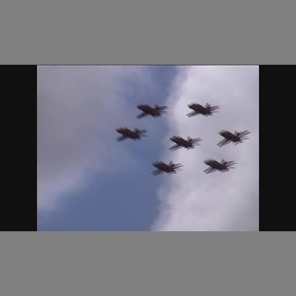
We can now randomly plot one of the detections.

detections_dir = "runs/detect/yolo_road_det/"
detection_images = [os.path.join(detections_dir, x) for x in os.listdir(detections_dir)]

random_detection_image = Image.open(random.choice(detection_images))
plt.imshow(np.array(random_detection_image))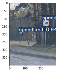

Apart from a folder of images, there are other sources we can use for our detector as well. The command syntax for doing so is described by the following.

python detect.py --source 0  # webcam
                            file.jpg  # image 
                            file.mp4  # video
                            path/  # directory
                            path/*.jpg  # glob
                            rtsp://170.93.143.139/rtplive/470011e600ef003a004ee33696235daa  # rtsp stream
                            rtmp://192.168.1.105/live/test  # rtmp stream
                            http://112.50.243.8/PLTV/88888888/224/3221225900/1.m3u8  # http stream

Computing the mAP on the test dataset

We can use the  test  file to compute the mAP on our test set. To perform the evaluation on our test set, we set the task flag to test. We set the name to yolo_det. Things like plots of various curves (F1, AP, Precision curves etc) can be found in the folder runs/test/yolo_road_det. The script calculates for us the Average Precision for each class, as well as mean Average Precision.

!python test.py --weights runs/train/yolo_road_det/weights/best.pt --data road_sign_data.yaml --task test --name yolo_det

The output of looks like the following:

Fusing layers... 
Model Summary: 224 layers, 7062001 parameters, 0 gradients, 16.4 GFLOPS
test: Scanning '../Road_Sign_Dataset/labels/test' for images and labels... 88 fo
test: New cache created: ../Road_Sign_Dataset/labels/test.cache
test: Scanning '../Road_Sign_Dataset/labels/test.cache' for images and labels...
               Class      Images     Targets           P           R      mAP@.5
                 all          88         126       0.961       0.932       0.944         0.8
        trafficlight          88          20       0.969        0.75       0.799       0.543
                stop          88           7           1        0.98       0.995       0.909
          speedlimit          88          76       0.989           1       0.997       0.906
           crosswalk          88          23       0.885           1       0.983       0.842
Speed: 1.4/0.7/2.0 ms inference/NMS/total per 640x640 image at batch-size 32
Results saved to runs/test/yolo_det2

And that's pretty much it for this tutorial. In this tutorial, we trained YOLO v5 on a custom dataset of road signs. If you want to play around with the hyperparameters, or if you want to train on a different dataset, you can grab the Gradient Notebook for this tutorial as a starting point.

Conclusion... and a bit about the naming saga.

As promised earlier, I want to conclude my article with giving my two cents about the naming controversy YOLO v5 created.

YOLO's original developer abandoned its development owing to concerns about his research being used for military purposes. After that, multiple sets of people have come up with improvements to YOLO.

Afterwards, YOLO v4 was released in April 2020 by Alexey Bochkovskiy and others. Alexey was perhaps the most suitable person to do a sequel to YOLO, since he had been the long-time maintainer of the second most popular YOLO repo, which unlike the original version, also worked on Windows.

YOLO v4 brought a host of improvements, which helped it greatly outperform YOLO v3. But then Glenn Jocher, maintainer of the Ultralytics YOLO v3 repo (the most popular python port of YOLO) released YOLO v5, the naming of which drew reservations from a lot of members of the computer vision community.

Why? Because in a traditional sense, YOLO v5 doesn't bring any novel architectures / losses / techniques to the table. There is yet to be a research paper released for YOLO v5.

It, however, provides massive improvements in terms of how quickly people can integrate YOLO into their existing pipelines. The foremost thing about YOLO v5 is that it's written in PyTorch / Python, unlike the original versions from v1-v4, which are in C. This alone makes it much more accessible to people and companies working in the deep learning space.

Moreover, it introduces a clean way of defining experiments using modular config files, mixed precision training, fast inference, better data augmentation techniques, etc. In a way, it would be fine to call it v5 if we viewed YOLO v5 as a piece of software, rather than an algorithm. Maybe that's what Glenn Jocher had in mind when he named it v5. Nevertheless, many folks from the community, including Alexey, have vehemently disagreed and pointed out that it's wrong to call it YOLO v5 since performance-wise, it is still inferior to YOLO v4.

Here is a post that gives you a more detailed account of the controversy.

YOLOv5 Controversy — Is YOLOv5 Real?

Marvelous ain’t it…at how fast we are progressing in our research and technology. I mean to get the next generation of the popular object detection framework so soon after its predecessor was just…

The StartupRitesh Kanjee

What's your take on this? Do you think YOLO v5 should be called so? Do let us know in the comments or simply tweet at @hellopaperspace.