Bring this project to life
Object detection remains one of the most popular and immediate use cases for AI technology. Leading the charge since the release of the first version by Joseph Redman et al. with their seminal 2016 work, "You Only Look Once: Unified, Real-Time Object Detection", has been the YOLO suite of models. These object detection models have paved the way for research into using DL models to perform realtime identification of the subject and location of entities within an image.
Last year we looked at and benchmarked two previous iterations of this model framework, YOLOv6 and YOLOv7, and showed how to step by step fine-tune a custom version of YOLOv7 in a Gradient Notebook.
In this article, we will revisit the basics of these techniques, discuss what is new in the latest release YOLOv8 from Ultralytics, and walk through the steps for fine-tuning a custom YOLOv8 model using RoboFlow and Paperspace Gradient using the new Ultralytics API. At the end of this tutorial, users should be able to quickly and easily fit the YOLOv8 model to any set of labeled images in quick succession.
How does YOLO work?
To start, let's discuss the basics of how YOLO works. Here is a short quote breaking down the sum of the model's functionality from the original YOLO paper:
"A single convolutional network simultaneously predicts multiple bounding boxes and class probabilities for those boxes. YOLO trains on full images and directly optimizes detection performance. This unified model has several benefits over traditional methods of object detection." (Source)
As stated above, the model is capable of predicting the location and identifying the subject of multiple entities in an image, provided it has been trained to recognized these features before. It does this in a single stage by separating the image into N grids, each of size s*s. These regions are simultaneously parsed to detect and localize any objects contained within. The model then predicts bounding box coordinates, B, in each grid with a label and prediction score for the object contained within.
Putting these all together, we get a technology capable of each of the tasks of object classification, object detection, and image segmentation. Since the basic technology underlying YOLO remains the same, we can infer this is also true for YOLOv8. For a more complete breakdown of how YOLO works, be sure to check out our earlier articles on YOLOv5 and YOLOv7, our benchmarks with YOLOv6 and YOLOv7, and the original YOLO paper here.
What's new in YOLOv8?
Since YOLOv8 was only just released, the paper covering the model is not yet available. The authors intend to release it soon, but for now, we can only go off of the official release post, extrapolate for ourselves the changes from the commit history, and try to identify for ourselves the extent of the changes made between YOLOv5 and YOLOv8.
Architecture
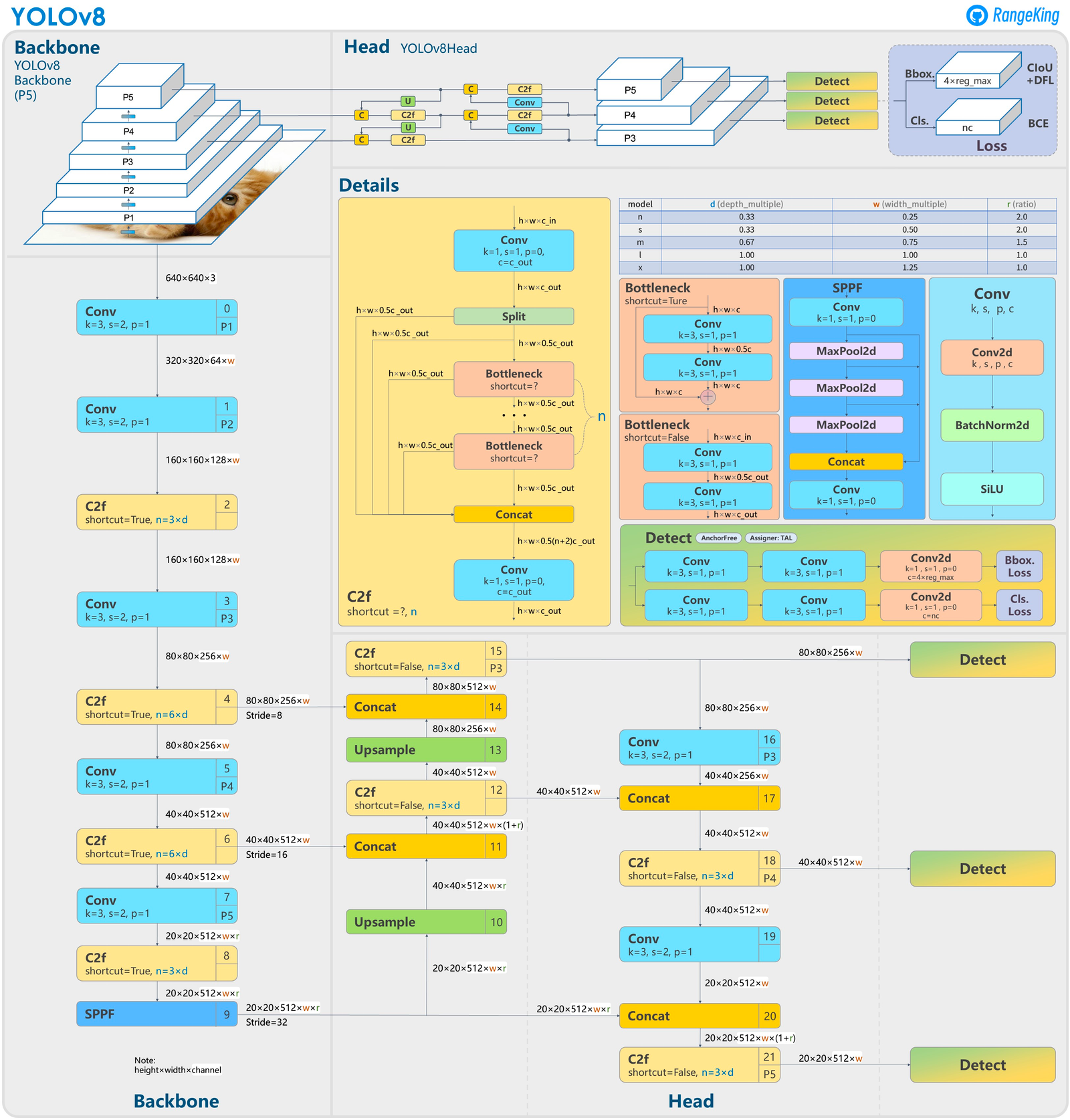
According to the official release, YOLOv8 features a new backbone network, anchor-free detection head, and loss function. Github user RangeKing has shared this outline of the YOLOv8 model infrastructure showing the updated model backbone and head structures. According to a comparison of this diagram with a comparable examination of YOLOv5, RangeKing identified the following changes in their post:
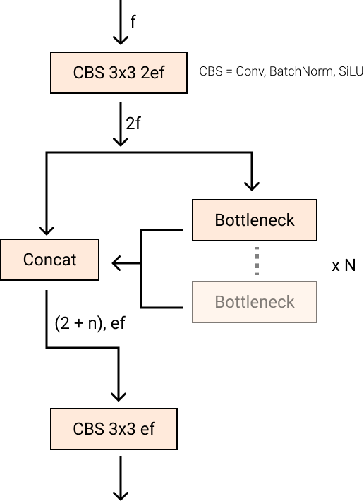
C2f module, credit to RoboFlow (Source)- They replaced the
C3module with theC2fmodule. InC2f, all the outputs from theBottleneck(the two 3x3convswith residual connections) are concatenated, but inC3only the output of the lastBottleneckwas used. (Source)
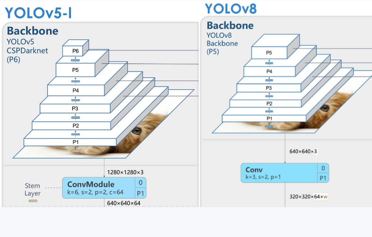
- They replaced the first
6x6 Convwith a3x3 Convblock in theBackbone - They deleted two of the
Convs (No.10 and No.14 in the YOLOv5 config)
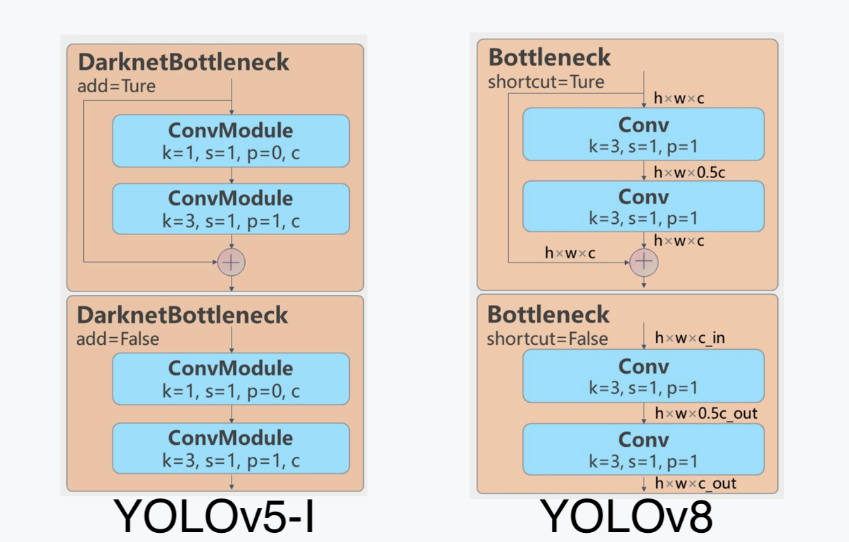
- They replaced the first
1x1 Convwith a3x3 Convin theBottleneck. - They switched to using a decoupled head, and deleted the
objectnessbranch
Check back here after the paper for YOLOv8 is released, we will update this section with additional information. For a thorough breakdown of the changes discussed above, please check out the RoboFlow article covering the release of YOLOv8
Accessibility
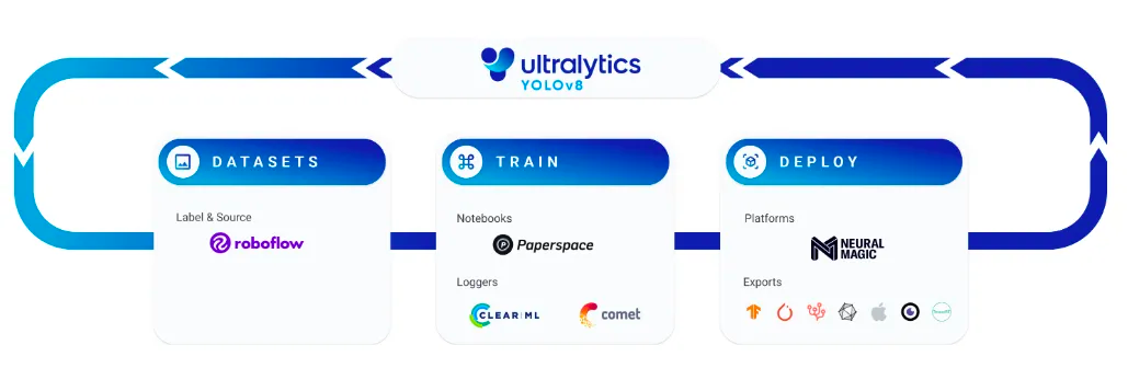
In addition to the old methology of cloning the Github repo, and setting up the environment manually, users can now access YOLOv8 for training and inference using the new Ultralytics API. Check out the Training your model section below for details on setting up the API.
Anchor free bounding boxes
According to Ultralytics partner RoboFlow's blog post covering YOLOv8, YOLOv8 now features the anchor free bounding boxes. In the original iterations of YOLO, users were required to manually identify these anchor boxes in order to facilitate the object detection process. These predefined bounding boxes of predetermined size and height capture the scale and aspect ratio of specific object classes in the data set. Calculating the offset from these boundaries to the predicted object helps the model better identify the location of the object.
With YOLOv8, these anchor boxes are automatically predicted at the center of an object.
Stopping the Mosaic Augmentation before the end of training
At each epoch during training, YOLOv8 sees a slightly different version of the images it has been provided. These changes are called augmentations. One of these, Mosaic augmentation, is the process of combining four images, forcing the model to learn the identities of the objects in new locations, partially blocking each other through occlusion, with greater variation on the surrounding pixels. It has been shown that using this throughout the entire training regime can be detrimental to the prediction accuracy, so YOLOv8 can stop this process during the final epochs of training. This allows for the optimal training pattern to be run without extending to the entire run.
Efficiency and accuracy
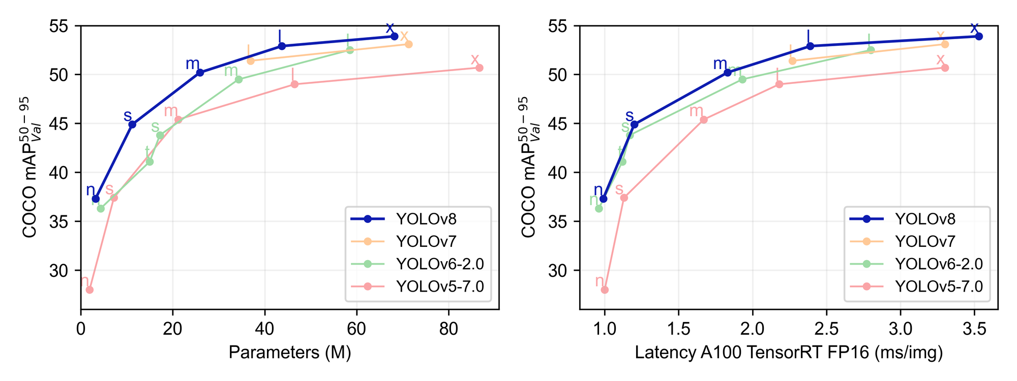
The main reason we are all here are the big boosts to performance accuracy and efficiency during both inference and training. The authors at Ultralytics have provided us with some useful sample data which we can use to compare the new release with other versions of YOLO. We can see from the plot above that YOLOv8 outperforms YOLOv7, YOLOv6-2.0, and YOLOv5-7.0 in terms of mean Average Precision, size, and latency during training.
| Model | size (pixels) | mAPval 50-95 | Speed CPU ONNX (ms) | Speed A100 TensorRT (ms) | params (M) | FLOPs (B) |
|---|---|---|---|---|---|---|
| YOLOv8n | 640 | 37.3 | 80.4 | 0.99 | 3.2 | 8.7 |
| YOLOv8s | 640 | 44.9 | 128.4 | 1.20 | 11.2 | 28.6 |
| YOLOv8m | 640 | 50.2 | 234.7 | 1.83 | 25.9 | 78.9 |
| YOLOv8l | 640 | 52.9 | 375.2 | 2.39 | 43.7 | 165.2 |
| YOLOv8x | 640 | 53.9 | 479.1 | 3.53 | 68.2 | 257.8 |
In their respective Github pages, we can find the statistical comparison tables for the different sized YOLOv8 models. As we can see from the table above, the mAP increases as the size of the parameters, speed, and FLOPs increase. The largest YOLOv5 model, YOLOv5x, achieved a maximum mAP value of 50.7. The 2.2 unit increase in mAP represents a significant improvement in capabilities. This is coserved across all model sizes, with the newer YOLOv8 models consistently outperforming YOLOv5, as shown by the data below.
| Model | size (pixels) | mAPval 50-95 | mAPval 50 | Speed CPU b1 (ms) | Speed V100 b1 (ms) | Speed V100 b32 (ms) | params (M) | FLOPs @640 (B) |
|---|---|---|---|---|---|---|---|---|
| YOLOv5n | 640 | 28.0 | 45.7 | 45 | 6.3 | 0.6 | 1.9 | 4.5 |
| YOLOv5s | 640 | 37.4 | 56.8 | 98 | 6.4 | 0.9 | 7.2 | 16.5 |
| YOLOv5m | 640 | 45.4 | 64.1 | 224 | 8.2 | 1.7 | 21.2 | 49.0 |
| YOLOv5l | 640 | 49.0 | 67.3 | 430 | 10.1 | 2.7 | 46.5 | 109.1 |
| YOLOv5x | 640 | 50.7 | 68.9 | 766 | 12.1 | 4.8 | 86.7 | 205.7 |
Overall, we can see that YOLOv8 represents a significant step up from YOLOv5 and other competing frameworks.
Fine-tuning YOLOv8
Bring this project to life
The process for fine-tuning a YOLOv8 model can be broken down into three steps: creating and labeling the dataset, training the model, and deploying it. In this tutorial, we will cover the first two steps in detail, and show how to use our new model on any incoming video file or stream.
Setting up your dataset
We are going to be recreating the experiment we used for YOLOv7 for the purpose of comparing the two models, so we will be returning to the Basketball dataset on Roboflow. Check out the "Setting up your custom datasets section" of the previous article for detailed instruction for setting up the dataset, labeling it, and pulling it from RoboFlow into our Notebook.
Since we are using a previously made dataset, we just need to pull the data in for now. Below is the command used to pull the data into a Notebook environment. Use this same process for your own labeled dataset, but replace the workspace and project values with your own to access your dataset in the same manner.
Be sure to change the API key to your own if you want to use the script below to follow the demo in the Notebook.
!pip install roboflow

from roboflow import Roboflow
rf = Roboflow(api_key="")
project = rf.workspace("james-skelton").project("ballhandler-basketball")
dataset = project.version(11).download("yolov8")
!mkdir datasets
!mv ballhandler-basketball-11/ datasets/
Training your model
With the new Python API, we can use the ultralytics library to facilitate all of the work within a Gradient Notebook environment. We will build our YOLOv8n model from scratch using the provided config and weights. We will then fine-tune it using the dataset we just loaded into the environment, using the model.train() method.
from ultralytics import YOLO

# Load a model
model = YOLO("yolov8n.yaml")  # build a new model from scratch
model = YOLO("yolov8n.pt")  # load a pretrained model (recommended for training)

# Use the model
results = model.train(data="datasets/ballhandler-basketball-11/data.yaml", epochs=10)  # train the model
Testing the model
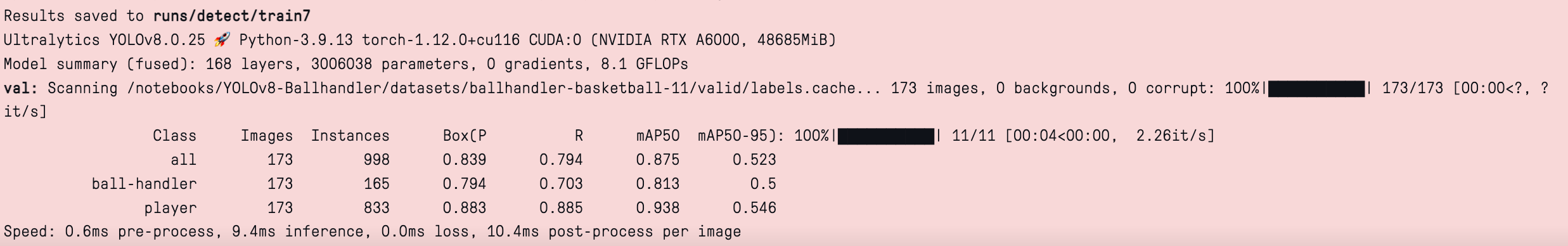
results = model.val() # evaluate model performance on the validation setWe can set our new model to evaluate on the validation set using the model.val() method. This will output a nice table showing how our model performed into the output window. Seeing as we only trained here for ten epochs, this relatively low mAP 50-95 is to be expected.
From there, it's simple to submit any photo. It will output the predicted values for the bounding boxes, overlay those boxes to the image, and upload to the 'runs/detect/predict' folder.
from ultralytics import YOLO
from PIL import Image
import cv2

# from PIL
im1 = Image.open("assets/samp.jpeg")
results = model.predict(source=im1, save=True)  # save plotted images
print(results)
display(Image.open('runs/detect/predict/image0.jpg'))
We are left with the predictions for the bounding boxes and their labels, printed like this:
[Ultralytics YOLO <class 'ultralytics.yolo.engine.results.Boxes'> masks
type: <class 'torch.Tensor'>
shape: torch.Size([6, 6])
dtype: torch.float32
 + tensor([[3.42000e+02, 2.00000e+01, 6.17000e+02, 8.38000e+02, 5.46525e-01, 1.00000e+00],
        [1.18900e+03, 5.44000e+02, 1.32000e+03, 8.72000e+02, 5.41202e-01, 1.00000e+00],
        [6.84000e+02, 2.70000e+01, 1.04400e+03, 8.55000e+02, 5.14879e-01, 0.00000e+00],
        [3.59000e+02, 2.20000e+01, 6.16000e+02, 8.35000e+02, 4.31905e-01, 0.00000e+00],
        [7.16000e+02, 2.90000e+01, 1.04400e+03, 8.58000e+02, 2.85891e-01, 1.00000e+00],
        [3.88000e+02, 1.90000e+01, 6.06000e+02, 6.58000e+02, 2.53705e-01, 0.00000e+00]], device='cuda:0')]
These are then applied to the image, like the example below:
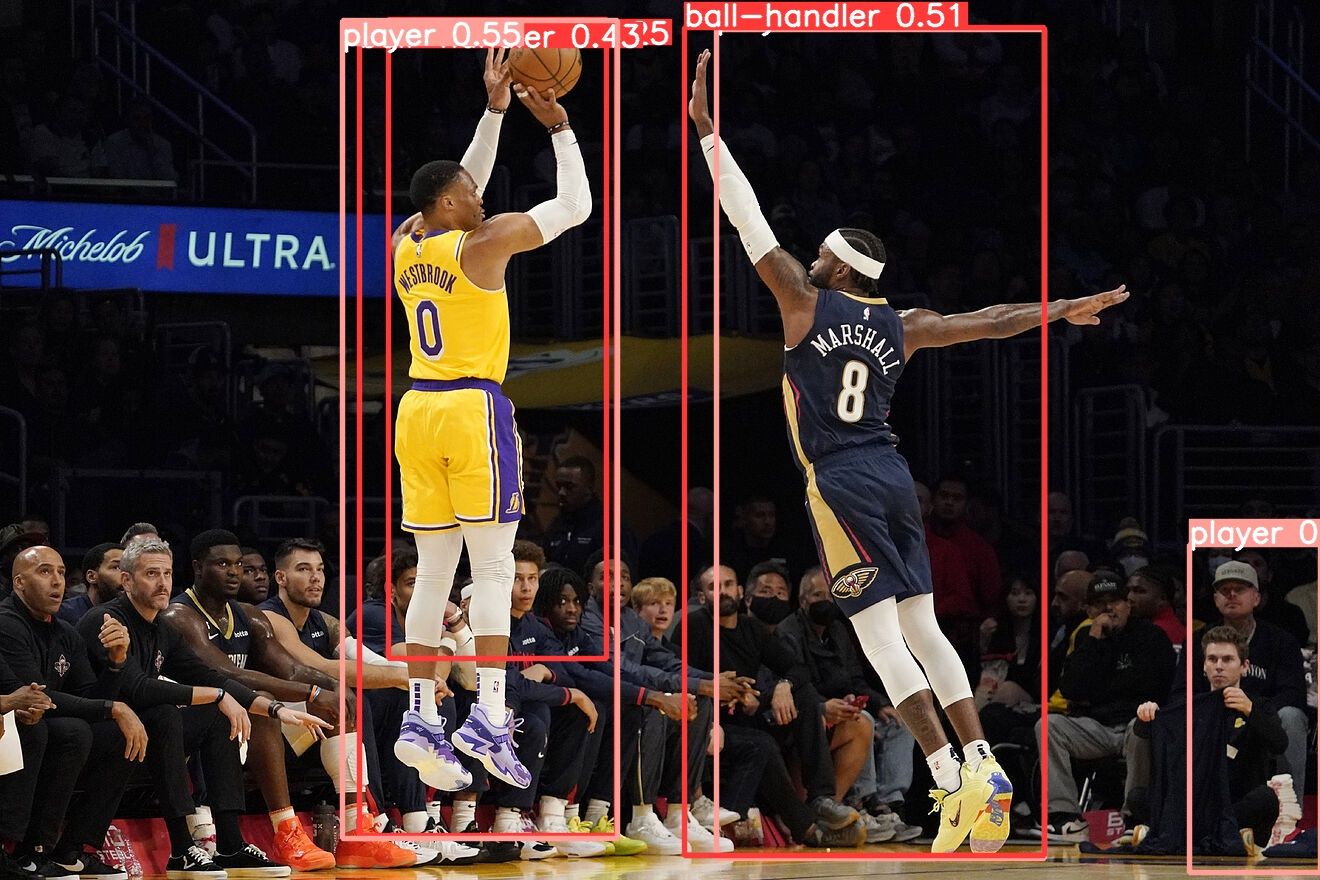
As we can see, our lightly trained model shows that it can recognize the players on the court from the players and spectators on the side of the court, with one exception in the corner. More training is almost definitely required, but it's easy to see that the model very quickly gained an understanding of the task.
If we are satisfied with our model training, we can then export the model in the desired format. In this case, we will export an ONNX version.
success = model.export(format="onnx") # export the model to ONNX formatClosing thoughts
In this tutorial, we examined what's new in Ultralytics awesome new model, YOLOv8, took a peak under the hood at the changes to the architecture compared to YOLOv5, and then tested the new model's Python API functionality by testing our Ballhandler dataset on the new model. We were able to show that this represents a significant step forward for simplifying the process of fine-tuning a YOLO object detection model, and demonstrated the capabilities of the model for discerning the possession of the ball in an NBA game using an in-game photo from the