
The quest for scene understanding in computer vision has led to many segmentation tasks. Panoptic segmentation is a new approach that combines semantic and instance segmentation into one framework.
This technique identifies each pixel captured within an image while distinguishing distinct instances belonging to the same object classes. This article will dive into the details of panoptic segmentation, applications, and challenges.
Panoptic Segmentation
Panoptic segmentation is a pretty interesting problem in computer vision these days. The goal is to split an image into two types - semantic regions and instance regions. The semantic areas are the parts of the image that belong to certain object classes, like a person or car. The instance regions are like the individual people or vehicles.
Unlike traditional semantic segmentation, which labels pixels as belonging to specific categories like "person" or "car," panoptic segmentation goes deeper. It labels pixels with their class and distinguishes between individual instances in the image. This approach aims to provide more information in a single output, a more detailed understanding of the scene than what traditional methods can do.
Task Format Explanation
Labels under “stuff” are continuous areas with no boundaries or countable features like sky, roadways, and grass. These regions are segmented using Fully Convolutional Networks (FCNs), which are good at segmenting broad background areas. The classification for distinct objects with recognizable features like people, cars, or animals falls under the label “thing.”
These objects are segmented using instance segmentation networks, which can identify and isolate individual instances. It can also assign a unique id to each object. This uses a dual labeling method to ensure all objects in the map have semantic information and precise instance delineation.
Introduction to the Panoptic Quality (PQ) Metric
The latest innovation in evaluation metrics is The Panoptic Quality (PQ). It was built to fix the problems with traditional segmentation evaluation methods. PQ is for panoptic segmentation, combining semantic and instance segmentation by assigning a class label and an instance ID to each pixel in the image.
Segment Matching Process
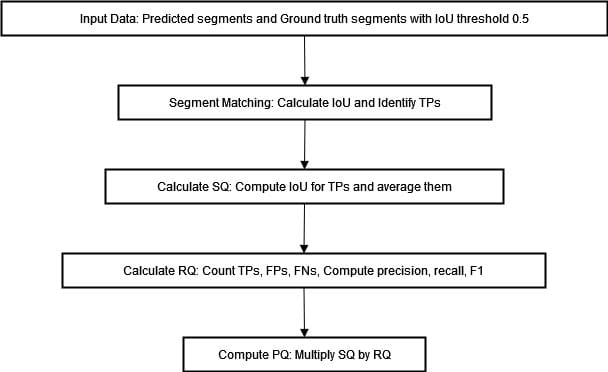
The initial step in the PQ metric computation is to perform a segment-matching process. This involves matching predicted segments with ground truth segments based on their Intersection over Union (IoU) values.
A match is deemed to have occurred when the Intersection over Union (IoU) value - a ratio that measures the overlap between predicted and ground truth segments - surpasses a predefined threshold commonly set at 0.5. This can be expressed in mathematical terms as follows:
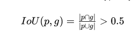
The threshold as mentioned above ensures that only those segments that demonstrate substantial overlap are regarded as viable matches. As a result, correctly segmented regions can be accurately identified while mitigating false positives and negatives.
PQ Computation
Upon successful matching of the segments, computation of the PQ metric ensues through an assessment of segmentation quality (SQ) and recognition quality(RQ).
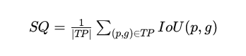
The segmentation quality (SQ) metric assesses the average intersection over union (IoU) of the match segments. It indicates how well the predicted segments overlap with the ground truth.
The recognition quality (RQ) measures the F1 score of the matched segments, balancing precision and recall.
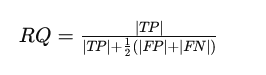
Here, TP stands for true positives, FP for false positives, and FN for false negatives. The PQ metric is then calculated as the product of these two components:
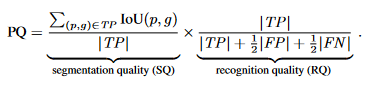
The formula above encapsulates the components of the PQ metric. We can visualize the process of computing PQ in the diagram below.
Advantages Over Existing Metrics
The PQ metric confers several benefits over existing metrics utilized for assessing segmentation tasks. Conventional metrics, such as mean Intersection over Union (mIoU) or Average Precision (AP), focus solely on semantic segmentation or instance segmentation individually, but not both.
The PQ metric presents a consolidated assessment framework that evaluates the performance of panoptic segmentation models. This approach proves especially advantageous for applications where thorough scene understanding is essential. Examples include autonomous driving and robotics. Object classification and individual instance identification assume pivotal significance in such scenarios.
Machine Performance on Panoptic Segmentation
State-of-the-art Panoptic Segmentation methods combine the latest instance and semantic segmentation techniques through a heuristic merging process.
The method starts by generating separate, non-overlapping predictions for things and stuff using the latest techniques. These are then combined to get a panoptic segmentation of the image.
In cases where there’s a conflict between thing and stuff prediction, our heuristic approach favors the thing class. This results in consistent performance for thing classes (PQTh) and slightly worse performance for stuff classes (PQSt).
Across various datasets, there are notable disparities when comparing machine performance with human consistency. On Cityscapes, ADE20k, and Mapillary Vistas, humans deliver superior results compared to machines.
The gap is especially evident in the Recognition Quality (RQ) metric, which measures F1 score accuracy. On the ADE20k dataset, humans get an RQ of 78.6%, and machines get around 43.2%.
The Segmentation Quality (SQ) metric, which measures the average IoU of matched segments, shows a smaller gap between humans and machine. Machines are getting better at segmentation but struggle to recognize and classify objects and regions.
| Dataset | Metric | Human | Machine |
|---|---|---|---|
| Cityscapes | PQ | 69.6 | 61.2 |
| SQ | 84.1 | 80.9 | |
| RQ | 82.0 | 74.4 | |
| ADE20k | PQ | 67.6 | 35.6 |
| SQ | 85.7 | 74.4 | |
| RQ | 78.6 | 43.2 | |
| Vistas | PQ | 57.7 | 38.3 |
| SQ | 79.7 | 73.6 | |
| RQ | 71.6 | 47.7 |
The table above shows the human vs machine performance across different datasets and metrics. The findings underscore critical areas where improvements are imperative for machines' Panoptic Segmentation algorithms.
Panoptic Segmentation Using DETR
we demonstrate how to explore the panoptic segmentation capabilities of DETR. The prediction occurs in several steps:
Bring this project to life
Installing the Required Packages and Importing the Necessary Libraries
The code below is a set of Python imports and configurations commonly used in computer vision and image-processing tasks.
from PIL import Image
import requests
import io
import math
import matplotlib.pyplot as plt
%config InlineBackend.figure_format = 'retina'

import torch
from torch import nn
from torchvision.models import resnet50
import torchvision.transforms as T
import numpy
torch.set_grad_enabled(False);
Install the COCO 2018 Panoptic Segmentation Task API
The following command installs the COCO 2018 Panoptic Segmentation Task API. This API is used to work with the COCO dataset, a large-scale object detection, segmentation, and captioning dataset.
pip install git+https://github.com/cocodataset/panopticapi.git
Import the COCO 2018 Panoptic Segmentation Task API and its Utility Functions
The code below imports the COCO 2018 Panoptic Segmentation Task API and its utility functions id2rgb and rgb2id.
id2rgb takes a panoptic segmentation map that uses ID numbers for each pixel and converts it into an RGB image. The input is a 2D array of integers that represent class IDs. The output is a 3D array of integers where each integer is the RGB color of the corresponding pixel. It’s converting from a map that shows what object or class each pixel represents to an image where we see the actual colors.
The rgb2id function converts a panoptic segmentation map from its RGB representation to an ID representation.
import panopticapi
from panopticapi.utils import id2rgb, rgb2id
Starting Point for Working with COCO Dataset and API
In the code below, the CLASSES list has all the names of the different objects in the COCO dataset. The coco2d2 dictionary converts the class IDs in the COCO dataset to a different numbering scheme used by the Detectron2 library. The transform is a PyTorch library that prepares images before they go into a model. It resizes to 800x800, turns into a tensor variable, and normalizes the pixel values using the mean and standard deviation of the ImageNet dataset.
# These are the COCO classes
CLASSES = [
    'N/A', 'person', 'bicycle', 'car', 'motorcycle', 'airplane', 'bus',
    'train', 'truck', 'boat', 'traffic light', 'fire hydrant', 'N/A',
    'stop sign', 'parking meter', 'bench', 'bird', 'cat', 'dog', 'horse',
    'sheep', 'cow', 'elephant', 'bear', 'zebra', 'giraffe', 'N/A', 'backpack',
    'umbrella', 'N/A', 'N/A', 'handbag', 'tie', 'suitcase', 'frisbee', 'skis',
    'snowboard', 'sports ball', 'kite', 'baseball bat', 'baseball glove',
    'skateboard', 'surfboard', 'tennis racket', 'bottle', 'N/A', 'wine glass',
    'cup', 'fork', 'knife', 'spoon', 'bowl', 'banana', 'apple', 'sandwich',
    'orange', 'broccoli', 'carrot', 'hot dog', 'pizza', 'donut', 'cake',
    'chair', 'couch', 'potted plant', 'bed', 'N/A', 'dining table', 'N/A',
    'N/A', 'toilet', 'N/A', 'tv', 'laptop', 'mouse', 'remote', 'keyboard',
    'cell phone', 'microwave', 'oven', 'toaster', 'sink', 'refrigerator', 'N/A',
    'book', 'clock', 'vase', 'scissors', 'teddy bear', 'hair drier',
    'toothbrush'
]

# Detectron2 uses a different numbering scheme, we build a conversion table
coco2d2 = {}
count = 0
for i, c in enumerate(CLASSES):
  if c != "N/A":
    coco2d2[i] = count
    count+=1

# standard PyTorch mean-std input image normalization
transform = T.Compose([
    T.Resize(800),
    T.ToTensor(),
    T.Normalize([0.485, 0.456, 0.406], [0.229, 0.224, 0.225])
])
Load the DETR Model for Panoptic Segmentation
The code below loads the DETR model for panoptic segmentation from the Facebook Research GitHub repository using the PyTorch Hub API. Here is an overview of the code:
model, postprocessor = torch.hub.load('facebookresearch/detr', 'detr_resnet101_panoptic', pretrained=True, return_postprocessor=True, num_classes=250)
model.eval();
Note: The image used here is taken from that source
Download and Open the Image
The code below downloads and opens an image from the COCO dataset using the Pillow library.
url = "http://images.cocodataset.org/val2017/000000281759.jpg"
im = Image.open(requests.get(url, stream=True).raw)- The
requests.get()function sends an HTTP GET request to the URL and retrieves the image data. Thestream=Trueargument specifies that the response should be streamed rather than downloaded simultaneously. - The
rawattribute of the response object is used to access the raw image data. - The
Image.open()function from the Pillow library is used to open the raw image data and create a newImageobject. TheImageobject can then perform various image processing and manipulation tasks.
Run the Prediction
The code img = transform(im).unsqueeze(0) is used to preprocess an image using a PyTorch transform and convert it to a tensor. The im variable contains the image data as a Pillow Image object.
# mean-std normalize the input image (batch-size: 1)
img = transform(im).unsqueeze(0)
out = model(img)
Plot the Predicted Segmentation Masks
The following code is related to plotting the predicted segmentation masks for objects detected in an image using the DETR model for panoptic segmentation. Here is an overview of the code.
# compute the scores, excluding the "no-object" class (the last one)
scores = out["pred_logits"].softmax(-1)[..., :-1].max(-1)[0]
# threshold the confidence
keep = scores > 0.85

# Plot all the remaining masks
ncols = 5
fig, axs = plt.subplots(ncols=ncols, nrows=math.ceil(keep.sum().item() / ncols), figsize=(18, 10))
for line in axs:
    for a in line:
        a.axis('off')
for i, mask in enumerate(out["pred_masks"][keep]):
    ax = axs[i // ncols, i % ncols]
    ax.imshow(mask, cmap="cividis")
    ax.axis('off')
fig.tight_layout()
This code first calculates the scores for the predicted masks, not including the no-object category. Then, it sets a threshold only to keep masks that scored higher than 0. 85 confidence. The remaining masks are plotted out in a grid with five columns, and the number of rows is figured based on how many masks met the threshold. The out variable passed in is assumed to be a dictionary with the predicted masks and logit values.
DETR's Postprocessor
# the post-processor expects as input the target size of the predictions (which we set here to the image size)
result = postprocessor(out, torch.as_tensor(img.shape[-2:]).unsqueeze(0))[0]
The above code takes the output out and runs it through a post-processor, generating a result. It passes the image size into the postprocessor function, which takes the intended prediction size as input and spits out a processed output. The result variable contains the processed output of the post-processor applied to the input image.
Visualization
The code below imports the itertools and seaborn libraries and creates a color palette using itertools.cycle and seaborn.color_palette(). It then opens a special-format PNG file and retrieves the IDs corresponding to each mask. Finally, it colors each mask individually using the color palette and displays the resulting image using matplotlib. We can do a simple visualization of the result
import itertools
import seaborn as sns
palette = itertools.cycle(sns.color_palette())

# The segmentation is stored in a special-format png
panoptic_seg = Image.open(io.BytesIO(result['png_string']))
panoptic_seg = numpy.array(panoptic_seg, dtype=numpy.uint8).copy()
# We retrieve the ids corresponding to each mask
panoptic_seg_id = rgb2id(panoptic_seg)

# Finally we color each mask individually
panoptic_seg[:, :, :] = 0
for id in range(panoptic_seg_id.max() + 1):
  panoptic_seg[panoptic_seg_id == id] = numpy.asarray(next(palette)) * 255
plt.figure(figsize=(15,15))
plt.imshow(panoptic_seg)
plt.axis('off')
plt.show()
Output:

Panoptic Segmentation with Detectron2
In this section, we demonstrate how to obtain a better-looking visualization by leveraging Detectron2's plotting utilities.
Import Libraries
The code below installs detectron2 from its GitHub repository. The Visualizer class from the utils module of detectron2 is imported to facilitate efficient visualization of detection results. The MetadataCatalog from the data module of detectron2 is imported to access metadata pertaining to datasets.
# Install detectron2
pip install 'git+https://github.com/facebookresearch/detectron2.git'
from copy import deepcopy
import io
import numpy as np
import torch
from PIL import Image
import matplotlib.pyplot as plt
from detectron2.data import MetadataCatalog
from detectron2.utils.visualizer import Visualizer
Visualizing Panoptic Segmentation Predictions with DETR and Detectron2
This code extracts and processes segmentation data from DETR's predictions, adjusting class IDs to match detectron2. It defines the rgb2id function, copies segment info, reads the panoptic result from a PNG image, and converts it into an ID map using numpy and torch. Class IDs are then converted to align with detectron2's COCO format before visualizing the results using detectron2's Visualizer.
# Define the rgb2id function
def rgb2id(color):
if isinstance(color, np.ndarray) and len(color.shape) == 3:
color = color.astype(np.int32)
return color[:, :, 0] + 256 * color[:, :, 1] + 256 * 256 * color[:, :, 2]
return color
# We extract the segments info and the panoptic result from DETR's prediction
segments_info = deepcopy(result["segments_info"])
# Panoptic predictions are stored in a special format png
panoptic_seg = Image.open(io.BytesIO(result['png_string']))
final_w, final_h = panoptic_seg.size
# We convert the png into a segment id map
panoptic_seg = np.array(panoptic_seg, dtype=np.uint8)
panoptic_seg = torch.from_numpy(rgb2id(panoptic_seg))
# Detectron2 uses a different numbering of coco classes, here we convert the class ids accordingly
meta = MetadataCatalog.get("coco_2017_val_panoptic_separated")
for i in range(len(segments_info)):
c = segments_info[i]["category_id"]
segments_info[i]["category_id"] = meta.thing_dataset_id_to_contiguous_id[c] if segments_info[i]["isthing"] else meta.stuff_dataset_id_to_contiguous_id[c]
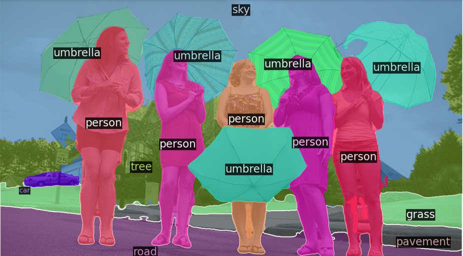
# Finally we visualize the prediction
v = Visualizer(np.array(im.copy().resize((final_w, final_h)))[:, :, ::-1], meta, scale=1.0)
v._default_font_size = 20
v = v.draw_panoptic_seg_predictions(panoptic_seg, segments_info, area_threshold=0)
# Display the image using matplotlib
result_img = v.get_image()
plt.figure(figsize=(12, 8))
plt.imshow(result_img)
plt.axis('off') # Turn off axis
plt.show()Output:
Conclusion
Panoptic segmentation represents a notable leap forward in the computer vision field by unifying semantic and instance segmentation under a consolidated framework. This approach affords an extensive understanding of scenes through pixel labeling and differentiation between diverse instances of similar object classes.
Panoptic Quality (PQ) metrics help to evaluate the effectiveness of panoptic models while identifying areas for improvement. While progress has been made, machine performance falls short compared to human consistency.
Integrating DETR and Detectron2 highlights how further developments can be leveraged towards autonomous driving or robotics applications.


