Translation Invariance & Equivariance in Convolutional Neural Networks

It's common knowledge that in a convolutional neural network, the processes of convolution and pooling work together in order to archive a final model objective. However, there are some quite beneficial bye-products of these two processes which are essential to the way convolutional neural networks process images; they are called translation invariance and translation equivariance.

#  article dependencies
import torch
import torch.nn as nn
import torch.nn.functional as F
import torchvision
import numpy as np
import matplotlib.pyplot as plt
import cv2
from tqdm.notebook import tqdm
import seaborn as sns
from torchvision.utils import make_grid

Translation in a Computer Vision Context

In a language context translation means interpretation of text or speech from one language to the other. However, in physics, translation (as in translational motion) simply means the movement of a body from one location to another on a spatial plane.

Translation in a computer vision context is more similar to the physics definition as translation of an object in an image implies the movement of that object from one location in the image to another. Consider the image below, the yellow pixel at index [2, 2] on the left is moved to index [7, 7], it can be said that the pixel has undergone translation from the top left corner to the bottom right corner.

Why It Matters

Using the images above as a point of reference, if the yellow pixel were to be shifted by just one pixel to the right (to index [2, 3]) a human would still probably see those images as essentially the same. However to a computer the two images will now be completely different; so from a computer vision point of view it is imperative to know how a convolutional neural network treats these two images based on translation of objects present in the image.  

Translation Equivariance

Equivariance in a mathematical context refers to a condition where a function provides the same output albeit with a different order when the order of the input upon which it acts on changes. Speaking contextually with regards to convolutional neural networks, translation equivariance implies that even when the position of an object in an image is changed the same features will be detected even at it's new position.

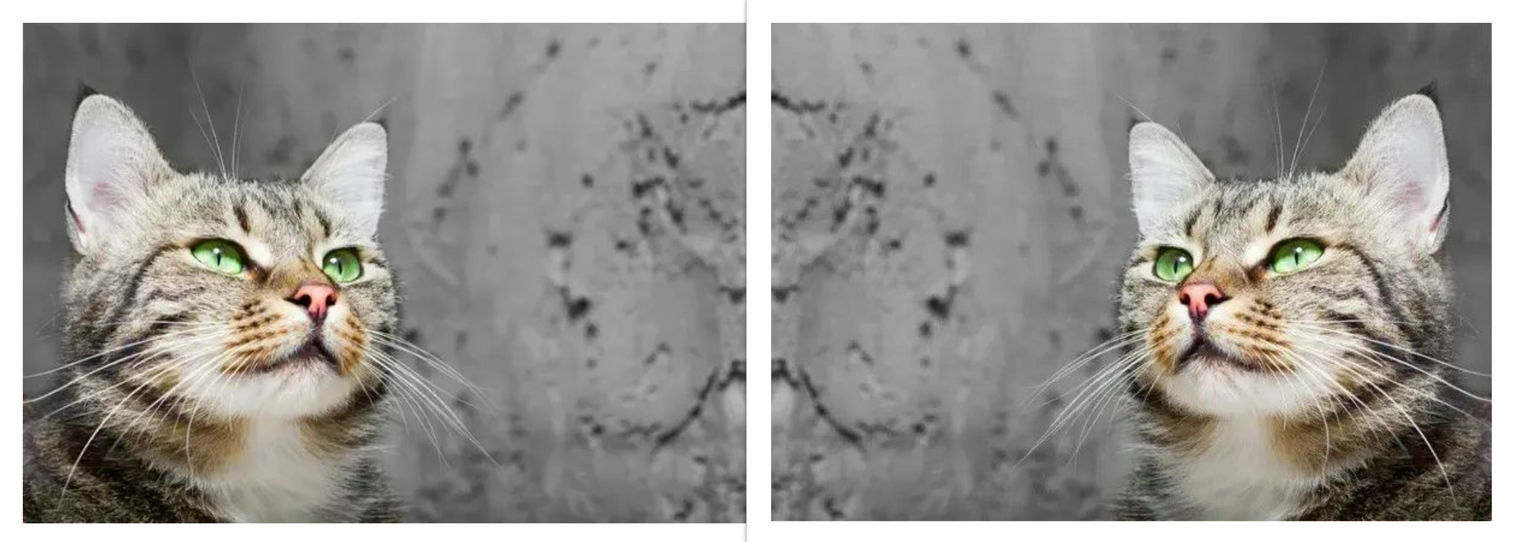
As you might have guessed, convolution layers will be responsible for this behavior as they are tasked with the burden of feature extraction. To investigate this, consider the image below, it is made of two distinct images with one being the mirrored version of the other. Using these images we will utilize the custom written convolution function, as defined in the code block below, in extracting features/detecting edges in the image.

def convolve(image_path, filter, title=''):
    """This function performs convolution over an image
    with the aim of edge detection"""

    if type(image_path) == np.ndarray:
      image = image_path
    else: 
      #  reading image
      image = cv2.imread(image_path, cv2.IMREAD_GRAYSCALE)

    #  defining filter size
    filter_size = filter.shape[0]

    #  creating an array to store convolutions
    convolved = np.zeros(((image.shape[0] - filter_size) + 1, 
                      (image.shape[1] - filter_size) + 1))
    
    #  performing convolution
    for i in tqdm(range(image.shape[0])):
      for j in range(image.shape[1]):
        try:
          convolved[i,j] = (image[i:(i+filter_size),
                                  j:(j+filter_size)] * filter).sum()
        except Exception:
          pass

    #  converting to tensor
    convolved = torch.tensor(convolved)
    #  applying relu activation
    convolved = F.relu(convolved)

    #  producing plots
    figure, axes = plt.subplots(1,2, dpi=120)
    plt.suptitle(title)
    axes[0].imshow(image, cmap='gray')
    axes[0].axis('off')
    axes[0].set_title('original')
    axes[1].imshow(convolved,)
    axes[1].axis('off')
    axes[1].set_title('convolved')
    return convolved

Using the above defined function, we will be detecting vertical edges in both images using the Sobel vertical edge detection filter outlined below.

#  defining sobel filter
sobel_y = np.array(([-1,0,1],
                    [-1,0,1],
                    [-1,0,1]))

#  detecting edges in image
convolve('image.jpg', filter=sobel_y)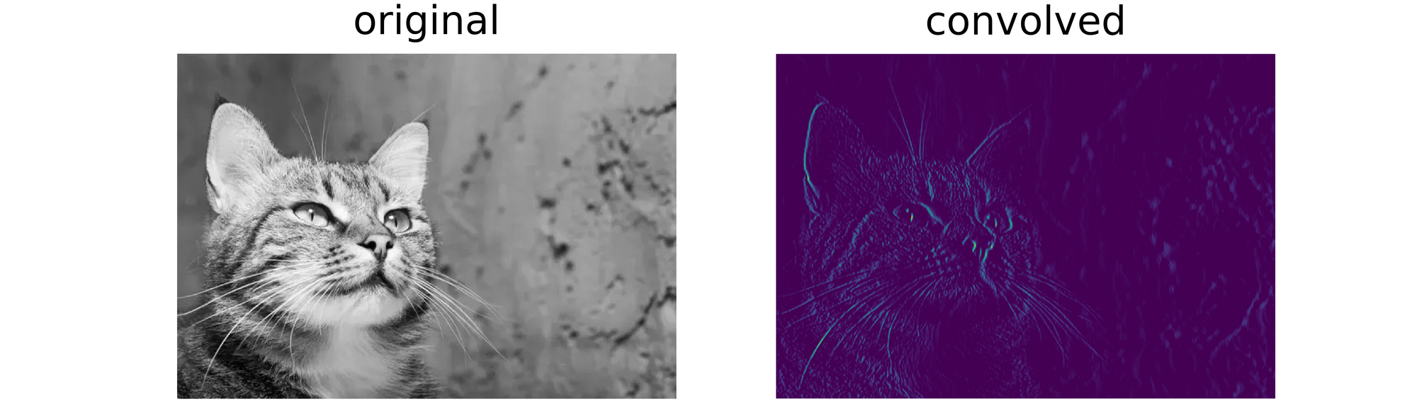

#  detecting edge in mirrored version of image
convolve('image_mirrored.jpg', filter=sobel_y)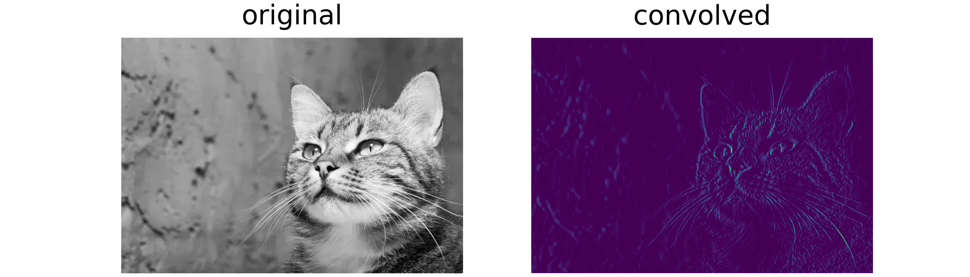

From the results obtained above, it is clear that although the position of the object of interest in the image had changed, the same edges were detected. This gives credence to the fact that convolutional neural networks, by virtue of their convolution layers, are in fact translation equivariant.

Translation Invariance

Translation invariance refers to a situation where a change in position of an object does not affect the nature of the output. Although they might sound contrasting, translation invariance and translation equivariance are not necessarily mutually exclusive, they can both occur at the same time although under different contexts as we will see below.

Unlike translation equivariance which is brought about by convolution operations in CNNs, translation invariance is a derivative of the pooling process. The whole idea is that even when an object of interest is moved around in an image, pooling brings the object into focus so that eventually their most salient features (pixels) end up in the same approximate location. To investigate this, consider the max pooling function written below, using this function we will be able to generate max pooled representations from images of interest.

def max_pool(image, kernel_size=2, visualize=False, title=''):
      """
      This function replicates the maxpooling
      process
      """

      #  assessing image parameter
      if type(image) is np.ndarray and len(image.shape)==2:
        image = image
      else:
        image = cv2.imread(image, cv2.IMREAD_GRAYSCALE)

      #  creating an empty list to store pooling
      pooled = np.zeros((image.shape[0]//kernel_size, 
                        image.shape[1]//kernel_size))
      
      #  instantiating counter
      k=-1
      #  maxpooling
      for i in tqdm(range(0, image.shape[0], kernel_size)):
        k+=1
        l=-1
        if k==pooled.shape[0]:
          break
        for j in range(0, image.shape[1], kernel_size):
          l+=1
          if l==pooled.shape[1]:
            break
          try:
            pooled[k,l] = (image[i:(i+kernel_size), 
                                j:(j+kernel_size)]).max()
          except ValueError:
            pass
            
      if visualize:
        #  displaying results
        figure, axes = plt.subplots(1,2, dpi=120)
        plt.suptitle(title)
        axes[0].imshow(image, cmap='gray')
        axes[0].set_title('reference image')
        axes[1].imshow(pooled, cmap='gray')
        axes[1].set_title('averagepooled')
      return pooled

The function below helps to iteratively apply the max pooling function on an image and return a visualization of both the reference image and it's max pooled representations.

def visualize_pooling(image, iterations, kernel=2, dpi=700):
      """
      This function helps to visualise several
      iterations of the pooling process
      """
      #image = cv2.imread(image, cv2.IMREAD_GRAYSCALE)

      #  creating empty list to hold pools
      pools = []
      pools.append(image)

      #  performing pooling
      for iteration in range(iterations):
        pool = max_pool(pools[-1], kernel)
        pools.append(pool)
      
      #  visualisation
      fig, axis = plt.subplots(1, len(pools), dpi=dpi)
      for i in range(len(pools)):
        axis[i].imshow(pools[i])
        axis[i].set_title(f'{pools[i].shape}', fontsize=5)
        axis[i].axis('off')
      pass

Image 1

Cast your mind back to the two images used to illustrate translation in one of the previous sections, lets attempt to recreate the one on the left with the yellow pixel located at the top left corner.

#  recreating image
image_1 = np.zeros((10, 10))
image_1[2, 2] = 1.0

Essentially, what we have done in the code cell above is to create a 10 x 10 matrix of zeros then we casted the pixel located at index [2, 2] to the value of 1 (This represents our yellow pixel.). From our knowledge of max-pooling, when using a (2, 2) kernel, we know it is a process whereby a filter is slid across 2 x 2 segments of the image and then the maximum value in that segment is returned as a pixel of it's own in a pooled representation.

Armed with that knowledge we can infer that if we go two max pooling representations deep for this particular image the yellow pixel will then be located at an index [0, 0] in a 2 x 2 pixel image. What has happened is that pooling has brought the most important feature in this particular image (the yellow pixel) into focus.

But don't take my word for it, let's actually max-pool the image using the functions we have written. From the result below, we can see that it does bare a striking resemblance to the hand drawn image.

visualize_pooling(image_1, 2, dpi=200)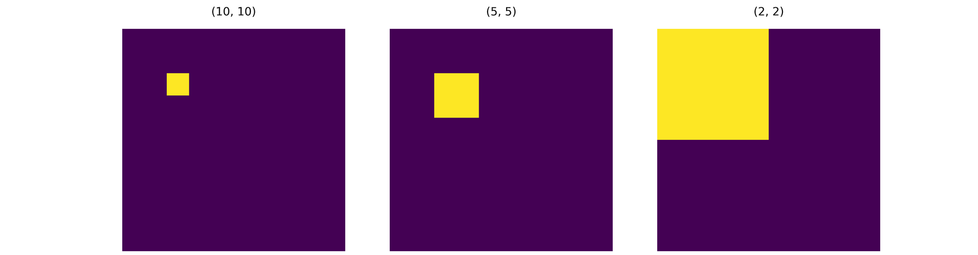

Image 2

Now let us attempt to recreate the second image on the right where the yellow pixel is located in the bottom right corner. In the same vane, when the image is max-pooled twice using a (2, 2) kernel then the yellow pixel will now be located at index [1, 1] as max pooling brings the most salient feature of the image into focus.

image_2 = np.zeros((10, 10))
image_2[-3, -3] = 1.0

Again, using the functions provided we can see that the resulting image bares a resemblance to the hand drawn illustration.

visualize_pooling(image_2, 2, dpi=200)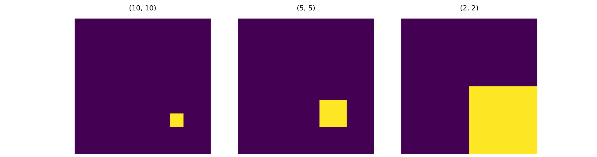

Comparing Images

Looking at the two reference images, the yellow pixels were originally five rows and five columns of pixels apart. However, after the first max-pooling process, the pixels became just two rows and two columns of pixels apart until they became just one row and one column apart by the second iteration of max-pooling. And of course, if max-pooling were to be performed one more time, only the yellow pixels will be returned in both instances.

This is essentially what translation invariance entails. Pooling make it such that regardless of where the object of interest might be moved to on the image, at the end of the day, it's features will be located in approximately the same position when max-pooled enough times.

Equivariance and Invariance Working in Tandem

In this section we will be taking a look at how translation equivariance and translation invariance work in tandem. In order to do this we will again be using the image in the next section as a reference image.

Reference Image

Using the reference image, we first need to detect edges in the image using the Sobel vertical edge detection filter previously defined. When this is done we then pass the detected edges as parameter to the pooling visualization function and go through 6 iterations of max pooling. The result is displayed below with the essential edges of the image being constrained into a 6 x 9 pixel image by the sixth iteration.

#  detecting edges in image
edges = convolve('image.jpg', filter=sobel_y)

#  going through 6 iterations of max pooling
visualize_pooling(np.array(edges), 6, dpi=500)

Mirrored Image

#  detecting edges in image
edges_2 = convolve('image_2.jpg', filter=sobel_y)

#  going through 6 iterations of max pooling
visualize_pooling(np.array(edges_2), 6, dpi=500)

Now using the mirrored version of the reference image and repeating the steps as outlined in the previous section produces the illustration that follows. From said illustration, we can see translation equivariance in action by virtue of the fact that the same exact features have been extracted even though the position of the object of interest has changed. Also, we can see translation invariance in action by lieu of the fact that although features are located in different positions, they are progressively brought toward the same position until they are in approximately the same location in a 6 x 9 pixel frame.

Comparison Image

Even when dealing with two completely different images, one can still see translation invariance in action. Consider the image above, when compared to the reference image, the object of interest in this image is located on the opposite side. However by the sixth epoch, it's most important features are also now located in the same approximate location as those of the reference image.

#  detecting edges in image
edges_3 = convolve('image_3.jpg', filter=sobel_y)

#  going through 6 iterations of max pooling
visualize_pooling(np.array(edges_3), 6, dpi=500)

Final Remarks

In this article. we have been able to look at two of the features of convolutional neural networks which make them quite robust. It's quite interesting that these two features have not actually been purposefully programed into the neural network rather they are bye products of processes that make a CNN what it it.