The Mechanics of Monocular Depth Estimation in Estimating Depth from 2D Images

Introduction

Depth Perception is a process of understanding 3D objects and judging how far these objects are. It helps in tasks like navigation, object manipulation, and scene understanding. Despite its importance, estimating depth from a single image, known as monocular depth estimation, is a challenging problem for Artificial Intelligence (AI) to solve.

However, advancements in machine learning, particularly deep learning or AI, have significantly improved the accuracy and reliability of monocular depth estimation. Convolutional Neural Networks (CNNs) and other deep learning architectures have shown great promise in learning to predict depth from 2D images by leveraging large datasets and powerful computational resources. These models are trained on diverse images with known depth information, allowing them to generalize to new, unseen scenes.

These techniques require diverse and extensive training data to be effective across various scenarios. However, gathering such data takes a lot of work. Sensors that provide detailed depth information, like structured light or time-of-flight sensors, have limitations in range and conditions. Laser scanners are expensive and only offer sparse depth measurements when moving objects are to be captured. On the other hand, stereo cameras show promise, but collecting enough stereo images in different environments is still a challenge.

As a result, researchers are exploring alternative approaches, such as using synthetic data, augmenting existing datasets, and employing techniques like structure-from-motion to create comprehensive training sets.

Structure-from-motion (SfM) methods have been used to create training data, but they need to capture moving objects, and there are gaps due to the limitations of multi-view matching. Currently, more than one dataset is required in order to train a model that can handle the variety found in real-world images. We have several datasets, each useful in some way but individually biased and incomplete. This highlights the need for more comprehensive datasets to improve monocular depth estimation models.

Understanding DPT: A Powerful Tool for Depth Estimation

Depth Anything model is based on the DPT architecture and has been trained on more than 62 million images. The backbone of the DPT model leverages a Vision Transformer(ViT) in place of CNN for dense prediction tasks, meaning predicting things per pixel.

DPT (Dense Prediction Transformer) is a novel architecture that estimates depth from a single image. It uses an encoder-decoder approach, where the encoder is based on the Vision Transformer (ViT), a significant advancement in computer vision. The encoder, also called the network's backbone, is pre-trained on a large corpus such as ImageNet.

The decoder aggregates features from the encoder and converts them to the final dense predictions.

Here's how it works: ViT uniquely processes the image, maintaining the same level of detail throughout and having a wide field of view. This helps DPT make detailed and globally consistent predictions. Instead of traditional methods that lose some detail through downsampling, DPT keeps the image quality high at all stages.

When monocular depth estimation and semantic segmentation were tested, DPT outperformed the leading convolutional networks by over 28%. It was especially effective on large datasets and even set new performance records on smaller ones like NYUv2 and KITTI. DPT excelled in semantic segmentation tasks, achieving top results on challenging datasets like ADE20K and Pascal Context.

The key to DPT's success is its ability to produce finer and more coherent predictions than traditional convolutional networks, making it a significant advancement in computer vision.

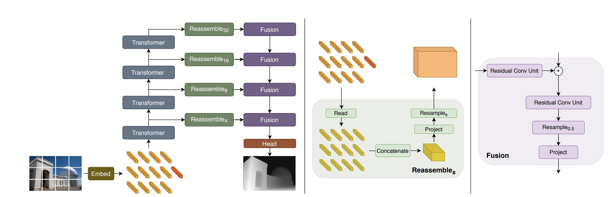
DPT Architecture

• Tokenization: The input image is converted into tokens either by:

1. Extracting non-overlapping patches and projecting them linearly (DPT-Base and DPT-Large), or
2. Using a ResNet-50 feature extractor (DPT-Hybrid).

• Embedding: The image tokens are augmented with positional embeddings and a readout token.
• Transformer Stages: The tokens pass through multiple transformer stages.
• Reassembly: Tokens from different stages are reassembled into image-like representations at multiple resolutions.
• Fusion and Upsampling: Fusion modules progressively combine and upsample these representations to create a fine-grained prediction. Fusion blocks use residual convolutional units to merge features and enhance the resolution.

To try the DPT model, go through the below steps:-

1. Set the environment

!pip install -q git+https://github.com/huggingface/transformers.git

2. Define the feature extractor and the model

from transformers import DPTFeatureExtractor, DPTForDepthEstimation

feature_extractor = DPTFeatureExtractor.from_pretrained("Intel/dpt-large")
model = DPTForDepthEstimation.from_pretrained("Intel/dpt-large")

3. Get the image

from PIL import Image
import requests

url = 'http://images.cocodataset.org/val2017/000000039769.jpg'
image = Image.open(requests.get(url, stream=True).raw)
image

4. Prepare the image

pixel_values = feature_extractor(image, return_tensors="pt").pixel_values
pixel_values

tensor([[[[ 0.1137,  0.1373,  0.1529,  ..., -0.1686, -0.2078, -0.1843],
          [ 0.0980,  0.1294,  0.2000,  ..., -0.2078, -0.1843, -0.2000],
          [ 0.1216,  0.1529,  0.1765,  ..., -0.1922, -0.1922, -0.2157],
          ...,
          [ 0.8275,  0.8353,  0.7882,  ...,  0.5059,  0.4510,  0.4196],
          [ 0.8039,  0.8196,  0.7490,  ...,  0.1843,  0.0745, -0.0353],
          [ 0.8667,  0.8196,  0.7098,  ..., -0.2471, -0.3333, -0.3804]],

         [[-0.8039, -0.8196, -0.8353,  ..., -0.9137, -0.8902, -0.9059],
          [-0.8039, -0.8039, -0.7804,  ..., -0.8824, -0.8980, -0.8824],
          [-0.7804, -0.7804, -0.7882,  ..., -0.8588, -0.8824, -0.8824],
          ...,
          [-0.2706, -0.2549, -0.2941,  ..., -0.5216, -0.5608, -0.5608],
          [-0.3176, -0.2863, -0.3333,  ..., -0.7020, -0.7490, -0.8275],
          [-0.2235, -0.2784, -0.3882,  ..., -0.8431, -0.8667, -0.8667]],

         [[-0.5373, -0.4824, -0.4510,  ..., -0.6941, -0.6941, -0.7176],
          [-0.5922, -0.5686, -0.4510,  ..., -0.6941, -0.7098, -0.7333],
          [-0.5922, -0.5373, -0.5373,  ..., -0.6941, -0.7176, -0.7569],
          ...,
          [ 0.5451,  0.5373,  0.4745,  ...,  0.2392,  0.2000,  0.1843],
          [ 0.6314,  0.5843,  0.5294,  ..., -0.1765, -0.2941, -0.3882],
          [ 0.4980,  0.5922,  0.5608,  ..., -0.6392, -0.6941, -0.6549]]]])

import torch

with torch.no_grad():
  outputs = model(pixel_values)
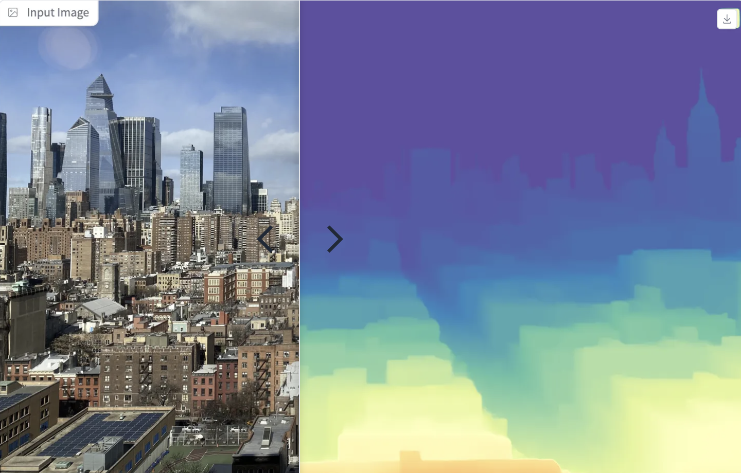
  predicted_depth = outputs.predicted_depth

5. Visualize the Image

import numpy as np

# interpolate to original size
prediction = torch.nn.functional.interpolate(
                    predicted_depth.unsqueeze(1),
                    size=image.size[::-1],
                    mode="bicubic",
                    align_corners=False,
              ).squeeze()
output = prediction.cpu().numpy()
formatted = (output * 255 / np.max(output)).astype('uint8')
depth = Image.fromarray(formatted)
depth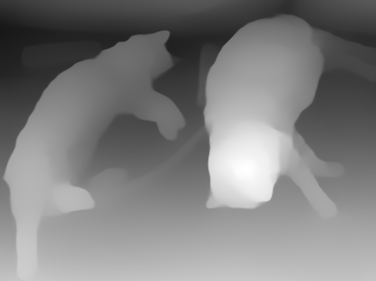

Depth Anything V2: A Look Back at the MIDAS Paper

Depth Anything V2 has achieved remarkable success in in-depth estimation, surpassing many other models and handling challenging images with impressive accuracy. To fully understand the capabilities of Depth Anything V2, it’s essential to revisit the foundational concepts introduced in the MIDAS paper from 2020.

MIDAS (Monocular Depth Estimation via a Multi-Scale Network) advanced the field by training a neural network to estimate depth from single images. It achieved this by leveraging diverse datasets, each contributing unique types of depth information. For example:

• KITTI Dataset: Focused on autonomous driving, this dataset provides images captured in outdoor environments using stereo cameras. These cameras are positioned at a fixed distance apart, allowing the extraction of depth information through post-processing techniques.
• NYU Depth V2 Dataset: Specializes in indoor scenes, capturing depth data through stereo imaging techniques in various household and office settings.

The MIDAS network was trained on these datasets to enhance its generalization ability across different scenes and conditions. By combining various sources of depth data, MIDAS learned to predict depth from a single image more accurately.

MiDaS

Monocular depth estimation, which determines the depth of objects from a single image, benefits from training on large and diverse datasets. However, collecting accurate depth information for many different environments is an impossible task, leading to various datasets with unique features and biases. To address this, we developed tools to combine multiple datasets during training, even if their depth annotations differ.

This paper introduced a novel loss function that we discussed later in the tutorial. This innovative loss function handles inconsistencies between datasets, such as unknown and varying scales and baselines. These losses allow training with data from different sensors, including stereo cameras (even with unknown calibration), laser scanners, and structured light sensors.

The extensive experiments demonstrate that a model trained on a diverse set of images with the proper training procedure achieves state-of-the-art results across various environments. The paper also focussed on zero-shot cross-dataset transfer to prove this, where the model is trained on specific datasets and tested on unseen ones. This method provides a more accurate measure of "real world" performance than training and testing on subsets of a single, biased dataset.

Advancements in Depth Anything V2

Building on the principles of MIDAS, Depth Anything has introduced several key improvements:

1. Enhanced Model Architecture: Depth Anything V2 uses a more advanced neural network architecture than MIDAS, incorporating recent developments in deep learning to improve depth prediction accuracy and handle more complex scenes.
2. High-Resolution Processing: Unlike earlier models that struggled with high-resolution inputs, Depth Anything V2 efficiently processes detailed images, enabling it to capture fine-grained depth information and handle intricate visual details.
3. Extended Training Datasets: Besides datasets like KITTI and NYU Depth V2, Depth Anything V2 utilizes additional datasets and synthetic data to further improve its robustness and accuracy across diverse environments.
4. Innovative Techniques: The model integrates novel techniques for handling occlusions, varying lighting conditions, and complex textures, which were challenging for earlier depth estimation models.
5. Real-World Applications: The advancements in Depth Anything V2 make it suitable for a wide range of applications, including autonomous driving, robotics, augmented reality (AR), and virtual reality (VR), where precise depth information is crucial.

Depth Anything

Depth Anything is a practical solution for robust monocular depth estimation. Depth Anything is a simple yet powerful foundational model capable of handling any image in any condition. The dataset is created using a data engine that collects and automatically annotates many unlabeled data (~62M), significantly increasing data coverage and reducing generalization errors.

Two effective strategies were used: creating a more challenging optimization target through data augmentation and developing auxiliary supervision to inherit rich semantic priors from pre-trained encoders. The models are evaluated on zero-shot capabilities using six public datasets and random photos, demonstrating impressive generalization. Fine-tuning with metric depth information from NYUv2 and KITTI data sets new state-of-the-art benchmarks.

Monocular depth estimation leverages large-scale unlabeled images instead of relying solely on costly and time-consuming methods like depth sensors, stereo matching, or Structure-from-Motion (SfM). The authors propose using monocular images, which are inexpensive and widely available, to build a robust MDE foundation model capable of producing high-quality depth information under various conditions.

They address the challenge of annotating these unlabeled images by designing a data engine that automatically generates depth labels using a pre-trained MDE model. This engine processes 62 million diverse, unlabeled images from large-scale datasets and enhances them with depth annotations through self-training.

Despite the advantages, the authors find that directly combining labeled and pseudo-labeled images initially yields limited improvements. To overcome this, they introduce a more challenging optimization strategy for learning pseudo labels and incorporate auxiliary semantic segmentation tasks to improve scene understanding. Additionally, they use DINOv2’s strong semantic capabilities to align features and boost MDE performance, resulting in a model that excels in both depth estimation and multi-task perception.

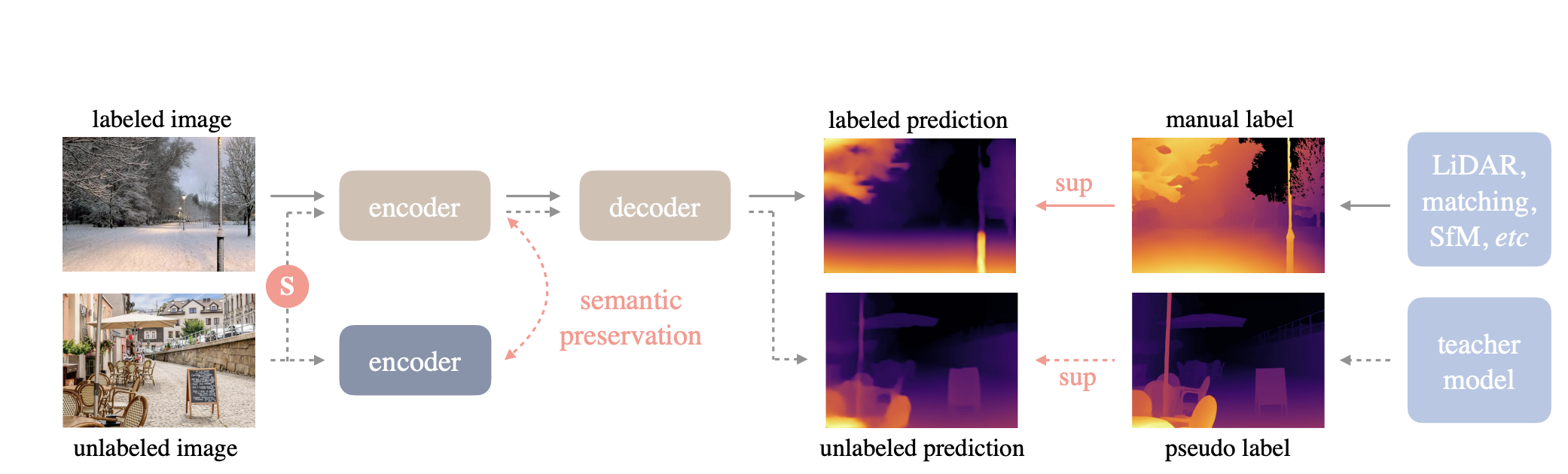
In this work, the authors improve monocular depth estimation (MDE) by leveraging both labeled and unlabeled images. They start by training a teacher model using a labeled dataset, where each image has a corresponding depth label. This teacher model is then used to generate pseudo depth labels for an unlabeled dataset. By doing so, the unlabeled images are effectively transformed into pseudo-labeled data. The next step involves training a student model on a combination of the original labeled dataset and the newly created pseudo-labeled dataset. This combined training approach enables the student model to learn from a much larger and more diverse set of data, enhancing its generalization capabilities and overall performance in depth estimation tasks.

The pipeline allows to use the model in a few lines of code:

from transformers import pipeline
from PIL import Image
import requests

# load pipe
pipe = pipeline(task="depth-estimation", model="LiheYoung/depth-anything-small-hf")

# load image
url = 'http://images.cocodataset.org/val2017/000000039769.jpg'
image = Image.open(requests.get(url, stream=True).raw)

# inference
depth = pipe(image)["depth"]

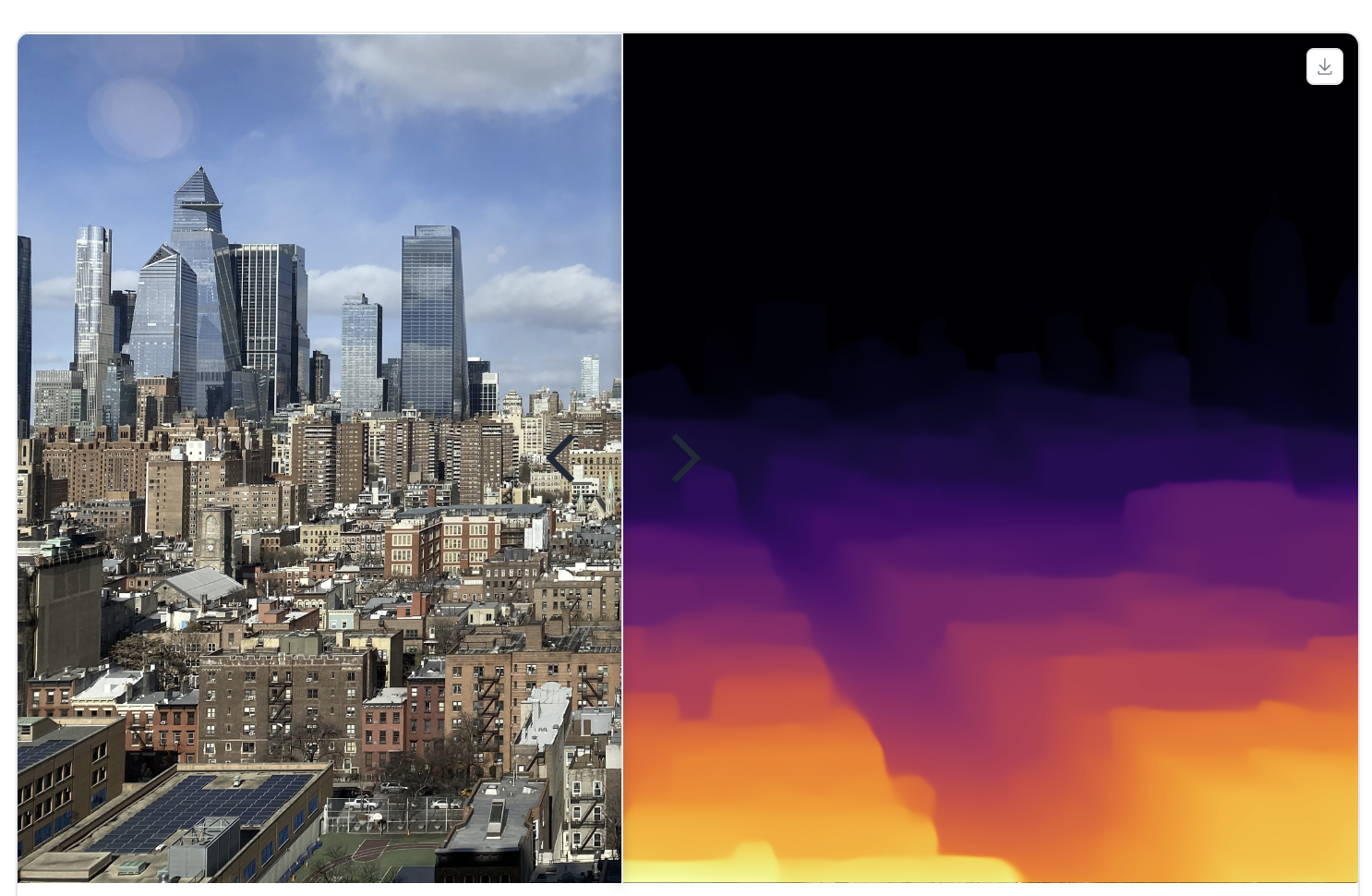
Depth Anything v2

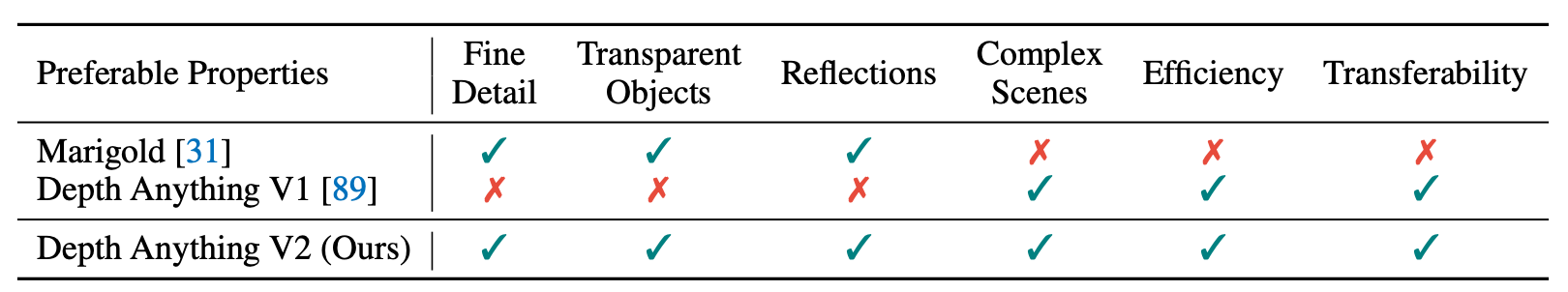
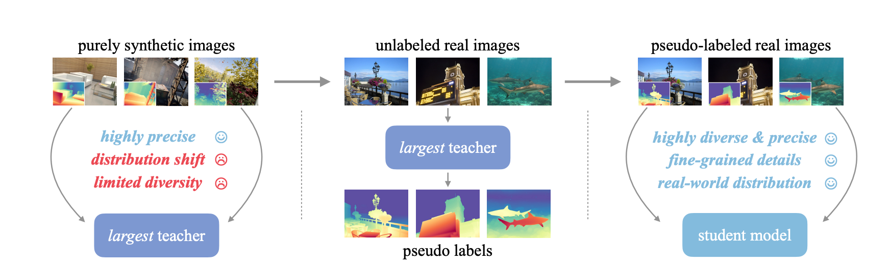
Depth Anything V2, a significant upgrade from V1, aimed to enhance the monocular depth estimation model. The main focus of this approach aims on improving three key points: using synthetic images instead of labeled real ones, increasing the capacity of our teacher model, and training student models with large-scale pseudo-labeled real images. These changes make the models not only faster—over ten times more efficient—than the latest Stable Diffusion-based models but also more accurate.

We have detailed blog on this model. Please click on the link to check out the blog!

The training pipeline for Depth Anything V2 is straightforward and involves three steps:

1. Train a reliable teacher model using DINOv2-G exclusively on high-quality synthetic images.
2. Generate accurate pseudo-depth labels for large-scale unlabeled real images.
3. Train the final student models on these pseudo-labeled real images to ensure robust generalization (demonstrating that synthetic images are not needed at this stage).

Loss Functions

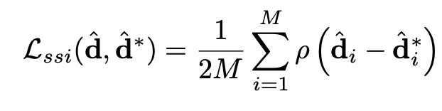
Training models for monocular depth estimation on diverse datasets is challenging due to varying forms of ground truth (absolute depth, scaled depth, or disparity maps). A suitable training scheme must operate in a compatible output space and use a flexible loss function to handle diverse data sources. The key challenges are: 1) Differing depth representations (direct vs. inverse), 2) Scale ambiguity (depth given up to an unknown scale), and 3) Shift ambiguity (disparity affected by unknown baseline and post-processing shifts).

Scale- and shift-invariant losses:- Scale- and shift-invariant losses for monocular depth estimation are methods designed to accurately measure the performance of a model, even when the depth data provided has uncertainties related to scale and shift. Here’s a simplified explanation:

1. Scale Invariance: In some datasets, the depth information is only provided up to an unknown scale, meaning we don't know the exact distances but rather the relative distances. A scale-invariant loss ensures that the model can still learn to estimate depth accurately without needing to know the exact scale. It focuses on the relative distances between objects, rather than their absolute distances.
2. Shift Invariance: Some datasets provide depth information (disparity maps) that might be shifted due to calibration issues or processing steps. A shift-invariant loss accounts for these shifts, allowing the model to learn the correct depth relationships without being thrown off by these unknown shifts.

These losses help the model focus on learning the true depth relationships in the scene, regardless of unknown scales or shifts in the input data, making it more robust and effective across diverse datasets.

Applications of Monocular Depth Estimation

Monocular depth estimation finds usefulness in a number of applications.

Here are some notable use cases:-

• Autonomous Vehicles: Depth estimation helps in identifying and avoiding obstacles for autonomous cars by providing a 3D understanding of the environment.
• Augmented Reality (AR) and Virtual Reality (VR): This model can serve well to create realistic 3D models for gaming or AR and VR experiences.
• Medical Imaging: Can be useful to assists in diagnosing conditions by analyzing depth-related changes in medical scans.
• Surveillance and Security: The ability to recognize and analyze activities by understanding the depth and movement of people.

Conclusions

Monocular depth estimation, utilizing just a single camera image to infer depth, has emerged as a transformative technology across diverse fields. Its ability to provide valuable information from 2D images enhances applications such as autonomous vehicles, where it helps in obstacle detection and navigation. As technology advances, monocular depth estimation is a strong algorithm to drive innovation and efficiency, making it a key component in the future of various industries.

References

• Depth Anything: Unleashing the Power of Large-Scale Unlabeled Data
• Towards Robust Monocular Depth Estimation: Mixing Datasets for Zero-shot Cross-dataset Transfer
• Depth Anything V2: A Powerful, Monocular Depth Estimation Model running on Paperspace H100 Machine Pricing
• Depth Anything V2