Introduction to Bagging and Ensemble Methods

The bias-variance trade-off is a challenge we all face while training machine learning algorithms. Bagging is a powerful ensemble method which helps to reduce variance, and by extension, prevent overfitting. Ensemble methods improve model precision by using a group (or "ensemble") of models which, when combined, outperform individual models when used separately.

In this article we'll take a look at the inner-workings of bagging, its applications, and implement the bagging algorithm using the scikit-learn library.

In particular, we'll cover:

• An Overview of Ensemble Learning
  • Why Use Ensemble Learning?
  • Advantages of Ensemble Learning
• What Is Bagging?
  • Bootstrapping
  • Basic Concepts
• Applications of Bagging
• The Bagging Algorithm
• Advantages and Disadvantages
• Decoding the Hyperparameters
• Implementing the Algorithm
• Summary and Conclusion

Let's get started.

An Overview of Ensemble Learning

As the name suggests, ensemble methods refer to a group of models working together to solve a common problem. Rather than depending on a single model for the best solution, ensemble learning utilizes the advantages of several different methods to counteract each model's individual weaknesses. The resulting collection should be less error-prone than any model alone.

Why Use Ensemble Learning?

Combining several weak models can result in what we call a strong learner.

We can use ensemble methods to combine different models in two ways:  either using a single base learning algorithm that remains the same across all models (a homogeneous ensemble model), or using multiple base learning algorithms that differ for each model (a heterogeneous ensemble model).

Generally speaking, ensemble learning is used with decision trees, since they're a reliable way of achieving regularization. Usually, as the number of levels increases in a decision tree, the model becomes vulnerable to high-variance and might overfit (resulting in high error on test data). We use ensemble techniques with general rules (vs. highly specific rules) in order to implement regularization and prevent overfitting.

Advantages of Ensemble Learning

Let’s understand the advantages of ensemble learning using a real-life scenario. Consider a case where you want to predict if an incoming email is genuine or spam. You want to predict the class (genuine/spam) by looking at several attributes individually: whether or not the sender is in your contact list, if the content of the message is linked to money extortion, if the language used is neat and understandable, etc. Also, on the other hand, you would like to predict the class of the email using all of these attributes collectively. As a no-brainer, the latter option works well because we consider all the attributes collectively whereas in the former one, we consider each attribute individually. The collectiveness ensures robustness and reliability of the result as it's generated after a thorough research.

This puts forth the advantages of ensemble learning:

• Ensures reliability of the predictions.
• Ensures the stability/robustness of the model.

To avail of these benefits, Ensemble Learning is often the most preferred option in a majority of use cases. In the next section, let’s understand a popular Ensemble Learning technique, Bagging.

What Is Bagging?

Bagging, also known as bootstrap aggregating, is the aggregation of multiple versions of a predicted model. Each model is trained individually, and combined using an averaging process. The primary focus of bagging is to achieve less variance than any model has individually. To understand bagging, let’s first understand the term bootstrapping.

Bootstrapping

Bootstrapping is the process of generating bootstrapped samples from the given dataset. The samples are formulated by randomly drawing the data points with replacement.

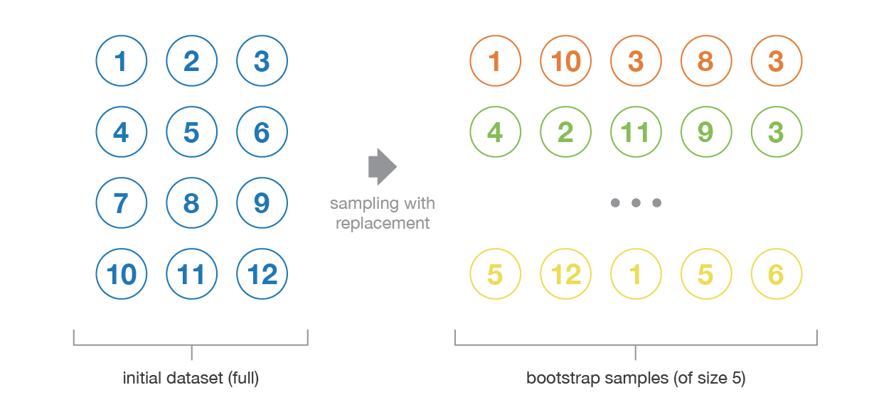
The resampled data contains different characteristics that are as a whole in the original data. It draws the distribution present in the data points, and also tend to remain different from each other, i.e. the data distribution has to remain intact whilst maintaining the dissimilarity among the bootstrapped samples. This, in turn, helps in developing robust models.

Bootstrapping also helps to avoid the problem of overfitting. When different sets of training data are used in the model, the model becomes resilient to generating errors, and therefore, performs well with the test data, and thus reduces the variance by maintaining its strong foothold in the test data. Testing with different variations doesn’t bias the model towards an incorrect solution.

Now, when we try to build fully independent models, it requires huge amounts of data. Thus, Bootstrapping is the option that we opt for by utilizing the approximate properties of the dataset under consideration.

Basic Concepts Behind Bagging

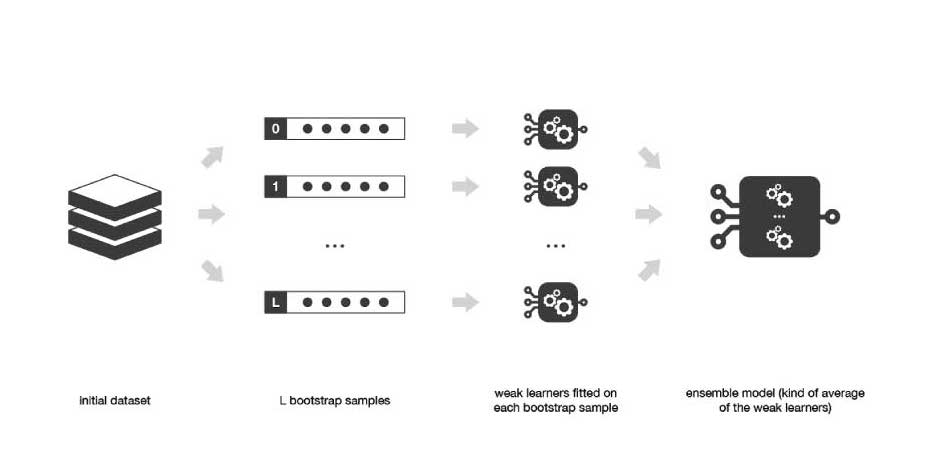
It all started in the year 1994, when Leo Breiman proposed this algorithm, then known as “Bagging Predictors”. In Bagging, the bootstrapped samples are first created. Then, either a regression or classification algorithm is applied to each sample. Finally, in the case of regression, an average is taken over all the outputs predicted by the individual learners. For classification either the most voted class is accepted (hard-voting), or the highest average of all the class probabilities is taken as the output (soft-voting). This is where aggregation comes into the picture.

Mathematically, Bagging is represented by the following formula,

The term on the left hand side is the bagged prediction, and terms on the right hand side are the individual learners.

Bagging works especially well when the learners are unstable and tend to overfit, i.e. small changes in the training data lead to major changes in the predicted output. It effectively reduces the variance by aggregating the individual learners composed of different statistical properties, such as different standard deviations, means, etc. It works well for high variance models such as Decision Trees. When used with low variance models such as linear regression, it doesn’t really affect the learning process. The number of base learners (trees) to be chosen depends on the characteristics of the dataset. Using too many trees doesn’t lead to overfitting, but can consume a lot of computational power.

Bagging can be done in parallel to keep a check on excessive computational resources. This is a one good advantages that comes with it, and often is a booster to increase the usage of the algorithm in a variety of areas.

Applications of Bagging

Bagging technique is used in a variety of applications. One main advantage is that it reduces the variance in prediction by generating additional data whilst applying different combinations and repetitions (replacements in the bootstrapped samples) in the training data. Below are some applications where the bagging algorithm is widely used:

• Banking Sector
• Medical Data Predictions
• High-dimensional data
• Land cover mapping
• Fraud detection
• Network Intrusion Detection Systems
• Medical fields like neuroscience, prosthetics, etc.

The Bagging Algorithm

Let’s look at the step-by-step procedure that goes into implementing the Bagging algorithm.

• Bootstrapping comprises the first step in Bagging process flow wherein the data is divided into randomized samples.
• Then fit another algorithm (e.g. Decision Trees) to each of these samples. Training happens in parallel.
• Take an average of all the outputs, or in general, compute the aggregated output.

It’s that simple! Now let’s talk about the pros and cons of Bagging.

Advantages and Disadvantages

Let’s discuss the advantages first. Bagging is a completely data-specific algorithm. The bagging technique reduces model over-fitting. It also performs well on high-dimensional data. Moreover, the missing values in the dataset do not affect the performance of the algorithm.

That being said, one limitation that it has is giving its final prediction based on the mean predictions from the subset trees, rather than outputting the precise values for the classification or regression model.

Decoding the Hyperparameters

Scikit-learn has two classes for bagging, one for regression (sklearn.ensemble.BaggingRegressor) and another for classification  (sklearn.ensemble.BaggingClassifier). Both accept various parameters which can enhance the model’s speed and accuracy in accordance with the given data. Some of these include:

base_estimator: The algorithm to be used on all the random subsets of the dataset. Default value is a decision tree.

n_estimators: The number of base estimators in the ensemble. Default value is 10.

random_state: The seed used by the random state generator. Default value is None.

n_jobs: The number of jobs to run in parallel for both the fit and predict methods. Default value is None.

In the code below, we also use K-Folds cross-validation. It outputs the train/test indices to generate train and test data. The n_splits parameter determines the number of folds (default value is 3).

To estimate the accuracy, instead of splitting the data into training and test sets, we use K_Folds along with the cross_val_score. This method evaluates the score by cross-validation. Here’s a peek into the parameters defined in cross_val_score:

estimator: The model to fit the data.

X: The input data to fit.

y: The target values against which the accuracy is predicted.

cv: Determines the cross-validation splitting strategy. Default value is 3.

Implementing the Bagging Algorithm

Step 1: Import Modules

Of course, we begin by importing the necessary packages which are required to build our bagging model. We use the Pandas data analysis library to load our dataset. The dataset to be used is known as the Pima Indians Diabetes Database, used for predicting the onset of diabetes based on various diagnostic measures.

Next, let's import the BaggingClassifier from the sklearn.ensemble package, and the DecisionTreeClassifier from the sklearn.tree package.

import pandas
from sklearn import model_selection
from sklearn.ensemble import BaggingClassifier
from sklearn.tree import DecisionTreeClassifier

Step 2: Loading the Dataset

We'll download the dataset from the GitHub link provided below. Then we store the link in a variable called url. We name all the classes of the dataset in a list called names.  We use the read_csv method from Pandas to load the dataset, and then set the class names using the parameter “names” to our variable, also called names. Next, we load the features and target variables using the slicing operation and assign them to variables X and Y respectively.

url="https://raw.githubusercontent.com/jbrownlee/Datasets/master/pima-indians-diabetes.data.csv"

names = ['preg', 'plas', 'pres', 'skin', 'test', 'mass', 'pedi', 'age', 'class']
dataframe = pandas.read_csv(url, names=names)
array = dataframe.values
X = array[:,0:8]
Y = array[:,8]

Step 3:  Loading the Classifier

In this step, we set the seed value for all the random states, so that the generated random values shall remain the same until the seed value is exhausted. We now declare the KFold model wherein we set the n_splits parameter to 10, and the random_state parameter to the seed value. Here, we shall build the bagging algorithm with the Classification and Regression Trees algorithm. To do so, we import the DecisionTreeClassifier, store it in the cart variable, and initiate the number of trees variable, num_trees to 100.

seed = 7
kfold = model_selection.KFold(n_splits=10, random_state=seed)
cart = DecisionTreeClassifier()
num_trees = 100

Step 4:  Training and Results

In the last step, we train the model using the BaggingClassifier by declaring the parameters to the values defined in the previous step.
We then check the performance of the model by using the parameters, Bagging model, X, Y, and the kfold model. The output printed will be the accuracy of the model.  In this particular case, it’s around 77%.

model = BaggingClassifier(base_estimator=cart,n_estimators=num_trees, random_state=seed)

results = model_selection.cross_val_score(model, X, Y, cv=kfold)
print(results.mean())

Output:

0.770745044429255

When using a Decision Tree classifier alone, the accuracy noted is around 66%. Thus, Bagging is a definite improvement over the Decision Tree algorithm.

Summary and Conclusion

Bagging improves the precision and accuracy of the model by reducing the variance at the cost of being computationally expensive. However, it is still a leading light in modeling a robust architecture. A model’s perfection doesn’t just attribute its success to the algorithm that is used, but also whether the algorithm being used is the right one!

Here’s a brief summary mentioning the notable points that we’ve learned about. We started off by understanding what ensemble learning is, followed by an introduction about bagging, moving on to its applications, working procedure, pros and cons, hyperparameters, and finally concluded by coding it in Python. Indeed, a good way to progress your Machine Learning skill!

References

https://towardsdatascience.com/ensemble-methods-bagging-boosting-and-stacking-c9214a10a205

https://bradleyboehmke.github.io/HOML/bagging.html#bagging-vip

https://en.wikipedia.org/wiki/Bootstrap_aggregating

https://scikit-learn.org/stable/modules/generated/sklearn.ensemble.BaggingClassifier.html

https://scikit-learn.org/stable/modules/generated/sklearn.model_selection.cross_val_score.html