“Net emissions of CO2 by human activities — including not only energy services and industrial production but also land use and agriculture — must approach zero in order to stabilize global mean temperature.” — Steven J. Davis et al., Net-zero emissions energy systems
Introduction
While the majority of energy consumptions remains dependent on conventional fossil fuels such as oil, natural gas, and coal, the emergence of renewable energy sources — such as wind, solar, biomass, geothermal, and hydropower — offer a sustainable solution to the current energy crisis.

The Challenge
Our supply chains currently contribute to over 80% of greenhouse gas emissions. Clearly, the optimization of our supply chains’ energy consumption is a key issue to address in order to make substantial strides toward a greener future.
Linear Programming: A Powerful Optimization Method
This article presents an optimization method, known as Linear Programming, to optimize the integration of renewable energy into existing supply chain infrastructure. Linear Programming (LP) is a powerful mathematical optimization method developed during World War II. The method provides a systematic and rigorous framework to facilitate complex decision-making, modeling linear relationships among variables to find the optimal solution.
The LP framework is composed of:
- The objective function-the linear function to be optimized.
- Decision variables-the variables whose optimal values comprise the final solution.
- The constraints-a set of linear inequalities that represent the restrictions imposed on the decision variables.
The objective is to find the set of values at which the decision variables yield the optimal solution, as specified by the objective function within the bounds of the linear constraints.
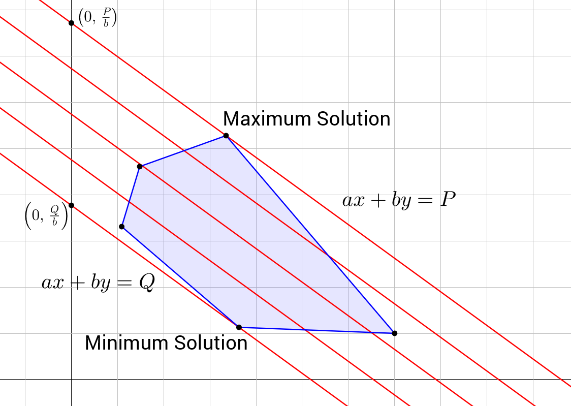
Simple 2-D linear programming problems can be solved graphically. This method offers a visual representation of the optimal solution, which can be found at the intersection of the linear objective function and the corner points of the feasible region. Pictured below, the red lines indicate the objective function’s level sets, which illustrate how varying decision variable values impact the final solution across differing expressions of the same objective function. The corner point selected as the optimal solution depends on whether we are maximizing or minimizing the objective function.
Case Study: Optimizing Renewable Energy Integration for a Multinational Computer Manufacturer Supply Chain
Now, let’s apply these principles to a more complex, real-world scenario. A large multinational company that manufactures computers currently consumes 100 MWh (megawatt– hours) of energy per day. Times are tough and the head of supply chain management has been granted just $25mil to reduce the company’s carbon footprint. Yikes! She is provided with the average estimated power output and cost estimates associated with implementing large, mid-size and small renewable energy power plants and tasked with maximizing the system’s renewable energy output.
Table 1: Megawatt-hours (expected value) produced by size j Power Plant powered by renewable energy source i
Table 2: Cost to build size j Power Plant powered by renewable energy source i
Leveraging Python’s PuLP Library for Optimization
To solve this problem, we can leverage Python’s PuLP library. This open-source resource provides a convenient and intuitive framework to formulate and solve optimization problems using Python.
# Install the library
# %pip install pulp

# Import the library
import pulp

# Formulate the problem
lp_problem = pulp.LpProblem('PowerGeneration', pulp.LpMinimize)

# Define the decision variables
## Size of Power Plant
sizes = ['Small', 'Mid-Size', 'Large']
## Type of Renewable Energy
sources = ["Hydropower", "Wind", "Solar", "Biomass", "Geothermal"]

x = pulp.LpVariable.dicts("Production", [(i, j) for i in sources for j in sizes], lowBound=0, cat=pulp.LpInteger)
# Generated power corresponding to each decision variable
gen_power = {
    ("Hydropower", 'Small'): 10,
    ("Hydropower", 'Mid-Size'): 20,
    ("Hydropower", 'Large'): 30,
    ("Wind", 'Small'): 0.25,
    ("Wind", 'Mid-Size'): 2,
    ("Wind", 'Large'): 3,
    ("Solar", 'Small'): 1,
    ("Solar", 'Mid-Size'): 5,
    ("Solar", 'Large'): 10,
    ("Biomass", 'Small'): 2,
    ("Biomass", 'Mid-Size'): 15,
    ("Biomass", 'Large'): 25,
    ("Geothermal", 'Small'): 8,
    ("Geothermal", 'Mid-Size'): 30,
    ("Geothermal", 'Large'): 50,
}
# Investment cost corresponding to each decision variable
inv_cost = {
    ("Hydropower", 'Small'): 2,
    ("Hydropower", 'Mid-Size'): 4,
    ("Hydropower", 'Large'): 6,
    ("Wind", 'Small'): 0.10,
    ("Wind", 'Mid-Size'): 1.5,
    ("Wind", 'Large'): 3,
    ("Solar", 'Small'): 1,
    ("Solar", 'Mid-Size'): 2,
    ("Solar", 'Large'): 3,
    ("Biomass", 'Small'): 1.5,
    ("Biomass", 'Mid-Size'): 2,
    ("Biomass", 'Large'): 3.5,
    ("Geothermal", 'Small'): 1,
    ("Geothermal", 'Mid-Size'): 3,
    ("Geothermal", 'Large'): 5,
}

# Define the objective function (maximize power)
objective = pulp.lpSum(gen_power[(source, size)] * x[(source, size)] for source in sources for size in sizes)
lp_problem += objective, "Maximize_Power"

# Define constraints
## Constraint 1: Total power generated must be at least 100
lp_problem += pulp.lpSum(gen_power[(source, size)] * x[(source, size)] for source in sources for size in sizes) >= 100, "Total_Power_Generated"
## Constraint 2: Total cost must be less than $25mil
lp_problem += pulp.lpSum(inv_cost[(source, size)] * x[(source, size)] for source in sources for size in sizes) < 25, "Total_Cost"

# Solve the linear programming problem
lp_problem.solve()
To generate more detailed information about our solution, we can code:
# Check the status of the solution
if pulp.LpStatus[lp_problem.status] == 'Optimal':
  print("Optimal Solution Found:")

# Initialize variables to store the total cost and power generated
total_cost = 0
total_power = 0

# Create a dict to store the breakdown of power sources and sizes
power_breakdown = {}

# Display the breakdown of power generated from each source
for source in sources:
  for size in sizes:
    source_power = x[(source, size)].varValue
    if source_power > 0:
      # Update the power breakdown dictionary
      power_breakdown[(source, size)] = source_power
      # Update the total cost and power
      total_cost += inv_cost[(source, size)] * source_power
      total_power += gen_power[(source, size)] * source_power

      # Print the detailed power breakdown dictionary
      for (source, size), power in power_breakdown.items():
        print(f"{size} {source} power plants: {power}")

      # Print the total power generated
      print(f"Total Power Generated: {total_power} MWh")

      # Print the total cost of the optimal solution
      print(f"Total Cost: ${total_cost}mil")
    else:
      print("No Optimal Solution Found")
This will give us our answers:
Optimal Solution Found.
- Small Wind power plants: 8.0
- Mid-Size Biomass power plants: 6.0
- Small Geothermal power plants: 1.0 units
______________________________
Total Power Generated: 100 MWh
Total Cost: $13.8mil
Coming in under budget?! Extra points.
Conclusion
By leveraging optimization techniques, we can address our toughest environmental and energy challenges. Supply chains, responsible for a significant share of greenhouse gas emissions, demand energy optimization. Linear Programming showcases math’s transformative potential, guiding us toward a cleaner, greener future.