AMPT-GA: Automatic Mixed Precision Floating Point Tuning for GPU Applications

Introduction

High-performance computing (HPC) scientific applications depend largely on floating-point arithmetic for high-precision outputs.
Certain variables may often be reduced in precision in these programs to speed up execution or minimize computing energy.
Recent NVIDIA GPUs perform single-precision floating-point operations at a throughput twice as fast than at double-precision. This trade-off becomes more significant when we strive to run large-scale applications, driven by increasing issue size. The accuracy of application outcomes, which must meet user-defined accuracy or error limits is critical. Mixed precision computing is the practice of combining various precisions for various floating-point variables. If we follow rules for determining accuracy, mixed precision training can greatly speed up any deep learning task.

The Way Towards Automatic Mixed Precision

Recent developments in the GPU sector have opened up new avenues for boosting performance. FP64 (double-precision) and FP16 (half-precision) arithmetic units have been added to GPUs, in addition to FP32(single precision). The upshot is that different performance levels may be achieved simultaneously using FP64/FP32/FP16 instructions.

Mixing FP64 and FP32 instructions had limited performance effect before these processors' release because mixed-precision math units were seldom available. Casting (or conversion) was required when selecting a mixed precision.

As an example of the utility of using mixed precision training, Baidu researchers have discovered considerable advancements in the area of LSTMs  used for voice recognition and machine translation employing a combination of FP32 and FP16 variables on a GPU with no change in accuracy.

Background on Prior Work

The paper we will base this blog post on can be found here: https://engineering.purdue.edu/dcsl/publications/papers/2019/gpu-fp-tuning_ics19_submitted.pdf

Here is some relevant background and prior work on mixed-precision optimization:

• As a first step, past works don't support the parallel codes present in GPU programming models since they depend on serial instrumentation or profiling assistance that doesn't span the GPU programming and execution paradigm, such as CPU-to-GPU calls.
• The second concern is that accuracy-centric techniques don't have a performance model and presume that the fastest running time is achieved with the least amount of precision. A mathematical operation can only be satisfied with the most precise operand if the mixing is accurate enough to be cast. Casting, on the other hand, is an expensive operation, so reducing precision may actually lengthen the time it takes to complete. There exist parallel pools of resources for FP64 and FP32 on many GPUs, and combining precision gives an extra parallelism opportunity that earlier work has ignored. To achieve overall accuracy criteria, precision levels have been established that typically fail to enhance the application's execution time.
• Lastly, methods that rely on real-time information  encounter issues related to search space. If the architecture supports three precision levels for the n floating-point variables that may be tweaked, the search space is (3 power n). Using this strategy in large production-level scientific applications, where n may reach hundreds of thousands, is impossible.

AMPT-GA:  A Mixed Precision Optimization System

To tackle a performance maximization challenge for GPU applications, AMPT-GA was developed. It is a mixed-precision optimization system. As determined by the program's end-user, the goal of AMPT-GA is to pick the set of precision levels for floating-point variables at an application level that improves performance while keeping the introduced error below an acceptable threshold. The Precision Vector (PV) is the final output of AMPT-GA, which assigns each floating-point variable to a precision level.

The main idea underlying AMPT-GA is that static analysis aids the dynamic search approach via the wide space of feasible precision vectors. In the paper, static analysis was used to identify groupings of variables whose precisions should be modified collectively to lessen the influence on the performance of any one variable's precision modification via casting. The broad search area may be sped up by such information. Researchers  employ  genetic algorithm for the search, which helps avoid the local minima that earlier techniques have a propensity to slip into.

The Paper's Claims to Innovation

• Using GPU-compatible static analysis in a genetic search method improves the efficiency of identifying viable mixed-precision programs.
  An execution filter based on a statically build performance model excludes precision vectors that cannot be profitable, therefore lowering the number of executions required by AMPT-GA in the course of its  search.
• Application-level precision guidance is provided by AMPT-GA instead of the localized kernels, functions, or instructions observed in past efforts.
• Experimentation has shown that our search technique can avoid local minima more effectively than current best practices, which results in significant time savings.

We find that AMPT-GA is able to outperform the state-of-the-art approach Precimonious by finding 77.1% additional speedup in LULESH’s mixed precision computations over its baseline of all double variables, while using a similar number of program executions as Precimonious. Our casting-aware static performance
model allows AMPT-GA to find precision combinations that Precimonious was unable to identify due to local minima issues. With three representative Rodinia benchmarks, LavaMD, Backprop, and CFD, we achieve additional speedups relative to Precimonious of 11.8%–32.9% when the tolerable error threshold is loose, and -5.9%–39.8% when the error threshold is the tightest. We choose these
three as they span the range of number and sizes of kernels as well as the spectrum of precisions available on latest generation GPU machines. We also evaluate the efficiency of the three solution approaches, which is the performance gain over the number of executions needed to search for the optimal PV, and AMPT-GA outperforms in this metric.

Source

It is worth noting that the US DOE (Department of Energy) uses Lulesh as a proxy app to benchmark large clusters since it represents many large codes.
It models hydrodynamics equations which explain the movement of materials with each other when subjected to forces. Researchers used the CUDA version of LULESH, with input size -s 50, and ran all experiments on a NVIDIA Tesla P100 GPU machine.

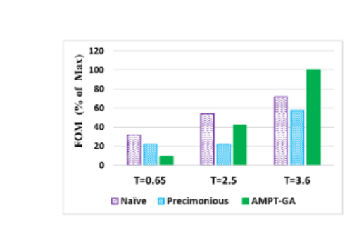
Studies were performed by changing the precision at the variable level for LULESH in the FP32 or FP64 space. FOM (Figure of Merit) were defined as the pace at which components in the simulation were processed.

It is a usual practice to output the FOM metric at the end of every LULESH code to measure overall performance. FOM is preferred over plain execution time for scaling reasons that are more esoteric, although the gains in wall-clock and FOM are directly proportional. The real statistic that was evaluated is the FOM as a percentage of the FOM with the lowest possible precision level.

It was found that compared to previous assessments, LULESH is a reasonably complex code encompassing 7,000 lines of C++ code on the GPU side and 600 LOC on the CPU side. A total of 76 floating-point variables were used for the test. Another important fact relating to the comparison: Precimonious, the most extensive program for which a mixed-precision solution could be obtained, contained 32 variables.

Five experiments were carried out in this research:

• Optimized Precision: In this experiment, researchers attempt to assess the relative execution benefit of AMPT-GA vis-á-vis the state-of-the-art Precimonious and naïve GA. We can see the results in figure a, figure b, figure c, and figure d.
• Error Threshold Adherence: This experiment confirms that the PVs picked in the preceding experiment fulfill the user-defined error constraint(See figure e).
• Component Testing: The purpose of this experiment was to investigate the effect of various components on the FOM metric(See figure f).
• Local vs. Global Models: The goal of this experiment was to quantify the advantage of applying application-level tuning versus kernel or function-level tuning (see table below).
• Precision Vector Generalization: In this experiment, the capacity to generalize to inputs within a narrow scope of the user-provided input value was tested (see figure g).

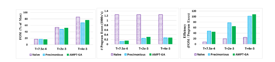
Researchers compare the application's performance after precision tuning using the FOM(Figure of Merit), which is synonymous with throughput and normalized to the FOM with all floats. AMPT-GA exceeds Precimonious for two of the three thresholds and outperforms the naïve solution for the top threshold. See the figure below.

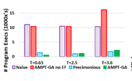
The number of executions for each protocol are shown in the figure below. Naïve, as expected, has the most number of executions, followed closely by AMPT-GA without the execution filter. The number of executions of AMPT-GA is either less or comparable to the number of Precimonious executions.

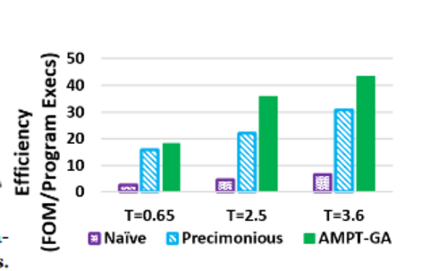
For all three error thresholds, AMPT-GA is the most efficient method, as shown below.

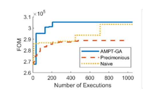
The figure below depicts the efficiency gain of each algorithm during a single program run. The results indicate that AMPT-GA can quickly converge to a higher FOM solution than the other two techniques. This occurs due to the GA's ability to make far more significant leaps than delta debugging(Delta debugging is more focused on local search).

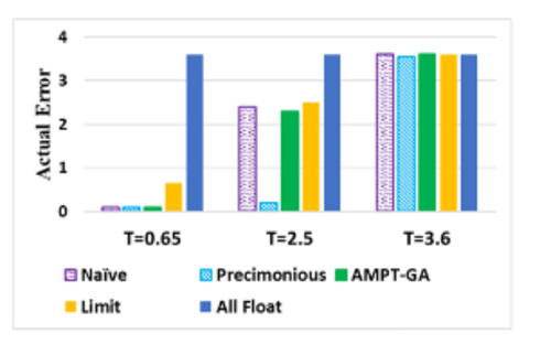
Each technique's performance and capacity to capitalize on available errors are shown in the figure below. These results show that all techniques, tight or flexible, fulfill the error constraints. Precimonious, on the other hand, is unable to make use of the available error headroom for the 2.5 thresholds.

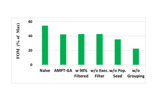
The FOM for the T=2.5 scenario is illustrated with various modules of AMPT-GA activated. The far-left scenario substitutes the performance model with actual program executions where it performs best, but at the expense of 10x extra executions. The grouping and hyper-dimensional space mutations have the highest impact, while the execution filter and the pre-population have a negligible effect for this particular error threshold. See the figure below.

The table below demonstrates the performance gain and error from the three kernels in LULESH, K1, K2, and K3, for a specific locally optimized precision vector.

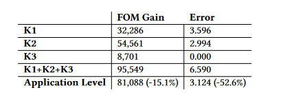
• There is an application-level shift in FOM and error due to the PV terms that affect K1 being all-floats, while the terms that affect K2 and K3 are all-doubles. K2 and K3 are treated similarly.
• If the kernel-level tweaking is adequate, the overall application FOM should equal a sum of the various kernel-level gains, but the application-level measure is 15.1 % lower.
• Compared to all of the individual kernel errors combined, the aggregate system error is far lower (52.6 %).

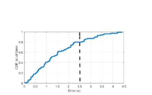
The error CDF is presented for the PV with a target error of 2.5 for inputs that are close the tested input. These findings suggest that most of the neighbors lie under the error limit, hence the result may be generalized with 80 % confidence. See the figure below.

Using Rodinia Benchmark Programs for Evaluation

As stated above, this approach was evaluated using three programs from the Rodinia GPU benchmark suite: LavaMD, Backprop, and CFD. LavaMD is a Molecular Dynamics program with a single kernel and 15 floating-point variables. Backprop is a two kernel benchmark with 21 floating-point variables that implement an algorithm in Pattern Recognition. CFD is a four kernel program with 26 floating-point variables that serve as a standard benchmark in Computational Fluid Dynamics. The results  obtained are as follows:

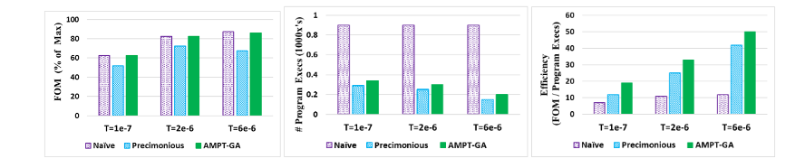
Results from LavaMD: the figure below shows that Naïve GA produces the greatest FOM values in all cases, although it requires a more significant proportion of program executions than the other approaches. AMPT-GA achieves a higher FOM than Precimonious.

Results from Backprop:  AMPT-GA achieves the same FOM values as Naïve GA while consuming less than a third of the number of executions. AMPT-GA is the most efficient method for all three error levels; you can see the figure below.

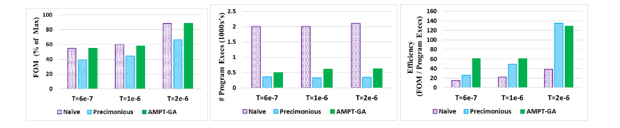
Results from CFD: The figure below shows that Naïve GA and AMPT-GA have the greatest FOM values in all scenarios; however, Naïve uses a far higher number of program executions than AMPT-GA.

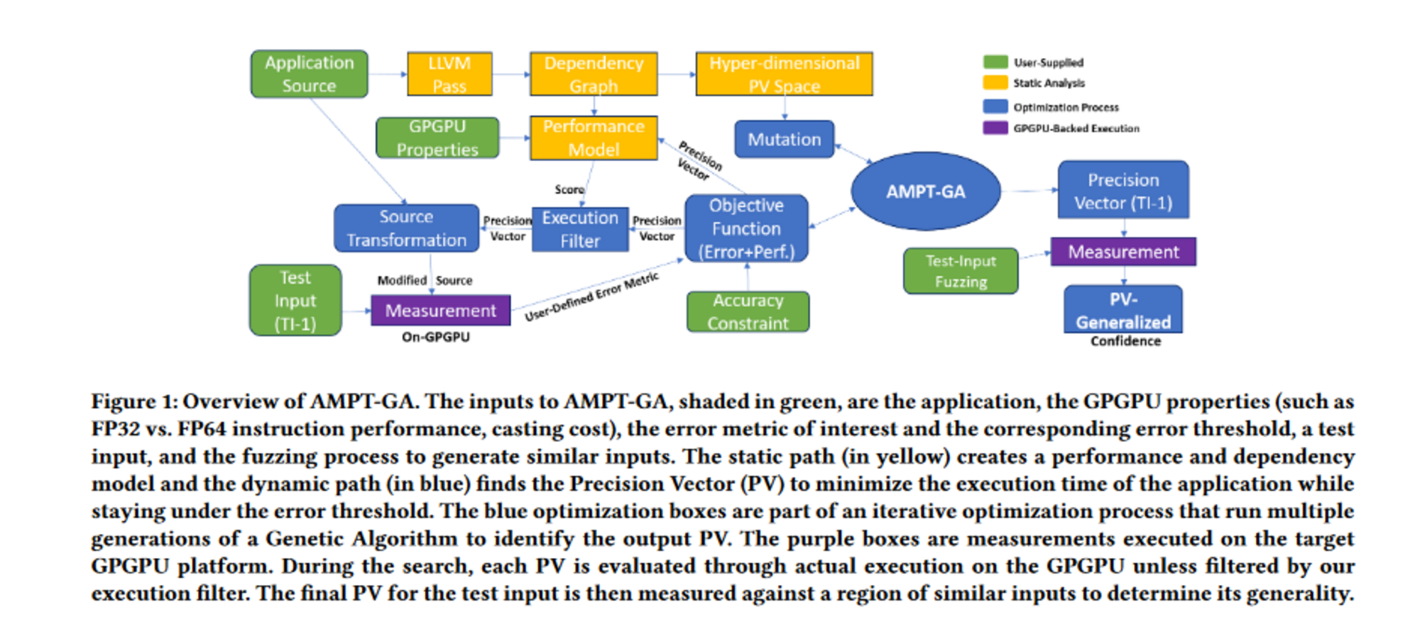
An Extensive Overview of The AMPT-GA

To use AMPT-GA, you need a test harness, an input from the target application or kernel, a list of variables that may be adjusted, and a specified error metric with its target error threshold (T). If a list of variables isn't provided, we'll use the application's floating-point variables or the kernel of a target GPU device to do the analysis. The paper assume that the architecture only handles instructions with inputs of the same precision.

• The building of the performance model must be done to predict the effect of reducing the precisions of the floating-point variables under consideration.
• Static analysis using an LLVM pass is used to build the model, which creates a dependency graph between the program's variables. The graph nodes are instructions and variable definitions, and the edges relate the definitions to their application in instruction.
• This graph, when given with the precision level for each variable, measures the number of operations of each precision and the number of castings that occur. This information is translated into a performance score that represents the relative performance due to quicker lower precision instructions among potential PVs.
• The dynamic execution parameters, such as the number of times a loop will be run, are not captured by this static pass since they are not changing.
  Although there is no assurance that the execution time of functions that have been given the same score would be the same, the score does offer a relative ranking of the potential for speedup among the various PVs.
• To find the PV with the highest performance while maintaining an error level below a certain threshold, we use a tweaked genetic algorithm (GA). This is because the PV space is binary restricted, the gradients between the PVs are not smooth, and the targets are non-linear in terms of error and performance.
• A point in the search space will only be executed if the predicted performance is better than the best obtained. The GA runs the program while taking into account the PV to find a certain point and then assesses the performance and error. This search point is rejected if it performs worse than the best performance so far (which will occur due to errors in our performance model) or if the error is greater than a threshold. Otherwise, it will be considered for selection in a future GA generation.
• To avoid casting penalties associated with dependent parameters (groups of related variables), the mutation function has been modified to change certain variables in the hyper-dimensional group space. Using GA, we can evaluate the best possible PV to use. The figure below illustrates how these various phases are intertwined.

• To reiterate an important point from above, We have to ask the GA to run an application with the current PV in mind, and because this is an expensive proposition (in comparison to querying our performance model), we will only do so if the performance model predicts that it will be a potentially worthwhile configuration.

The end-user workflow: For the deployment of AMPT-GA, the end-user must provide the application source, define a test input, and set a target threshold for error. AMPT-GA will determine the precision vector for all floating-point variables to optimize efficiency while achieving the threshold. It is possible to allow the end-user to choose which floating-point variables should be modified.

All of this can be run from with a Paperspace Core GPU powered machine to test it yourself directly.

Concepts About Operations of AMPT-GA

1. Operation of AMPT-GA: AMPT-GA is an optimization technique to pick the optimal precision vector (PV) to maximize performance while error is kept within the user-specified limit. We implement the constraint as an objective function penalty, such that erroneous solutions are rejected yet information about the degree of the error remains in the score to help guide the search.

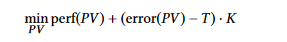
• perf (PV) is the performance score, and lower values indicate better performance
• error (PV) refers to the value of the error metric caused by the specified PV, while T is the threshold for this error metric
• K is a multiplicative factor with the following definition:
  1, if error (PV) ≤T and P, a large value greater than the maximum perf
  value, if error (PV)>T

2. User-Defined Error Metric. We use (by default) an application-generic error metric, which is the number of digits of precision compared to the most precise result.

3. Variables of Interest: Users may incorporate any floating point variables in an application, including arrays, structures, and individual variables. Those variables that are used in GPU kernels with high running times as determined by common profiling tools are selected in AMPT-GA.We start with the longest-running kernel, include it, and then work our way down the list according to running time. We terminate when we have included enough kernels to capture a certain proportion of overall program execution time. After a certain proportion of the overall program running time has been captured, we terminate our tests.

4. Black Box Search: A "black box" optimization procedure is used as a starting point for our search, which employs a genetic algorithm (GA) without any program analysis to guide the search.

5. Dependency Graph and Static Performance
Model: The performance gain from a specific PV may be estimated using the static performance model and the intermediate dependency graph. When a PV and application source code is supplied, the method estimates the amount of floating-point and double operations and casts that occur statically in the code. When estimating the number of casts and operation types in a compiled mixed-precision version of the program, the dependency graph is based on the program structure for the all-double scenario.

6. Precision Vector Optimization: AMPT-GA uses an optimization method to determine the best PV for the specified error threshold.

7. Execution Filtering: The error metric is measured and verified if it is below the threshold by AMPT-GA using the actual program executions. It implies that the application must first be executed to evaluate the objective function of a PV that has not yet been seen.

8. Program Transformation: In AMPT-GA, we must eventually apply the PV to the application such that the program's actual operations occur at the modified precision.

Conclusion

AMPT-GA is a solution for improving variable precision in applications using computationally intensive GPU kernels.  As a result of this, we have two innovations:

• A static analysis to identify variables that need to be changed simultaneously.
• A search technique that may quickly remove unprofitable PVs based on applicable penalties like type casting.

Reference: https://engineering.purdue.edu/dcsl/publications/papers/2019/gpu-fp-tuning_ics19_submitted.pdf