The success of Deep Learning models in Computer Vision tasks like image classification, semantic segmentation, object detection, etc., is attributed to taking advantage of the vast amounts of labeled data used for training a network - a method called supervised learning. Although a large amount of unstructured data is available in this era of Information Technology, annotated data is challenging to come by.
Data Labeling takes the majority of the time devoted to a computer vision Machine Learning project for this reason, and is also an expensive endeavor. Furthermore, in fields like healthcare, only expert doctors can categorize the data- for example, take a look at the following two images of cervical cytology- can you definitively say which one is cancerous?

Most untrained medical professionals will not know the answer- (a) is cancerous, while (b) is benign. So, data labeling is more difficult in such scenarios. At best, we would have only a handful of annotated samples, which is not nearly enough to train supervised learning models.
Also, newer data may gets incrementally available over time - like when data from a newly identified species of birds may become available. Training a deep neural network on a large dataset consumes a lot of computational power (for example, ResNet-200 took about three weeks to train on 8 GPUs). Having to retrain the model to accommodate the newly available data is therefore unfeasible in most scenarios.
This is where the relatively new concept of Few-Shot Learning comes in.
What is Few-Shot Learning?
Few-Shot Learning (FSL) is a Machine Learning framework that enables a pre-trained model to generalize over new categories of data (that the pre-trained model has not seen during training) using only a few labeled samples per class. It falls under the paradigm of meta-learning (meta-learning means learning to learn).
We, humans, are able to identify new classes of data easily using only a few examples using our previously learned knowledge. FSL aims to mimic the same. This is called meta-learning, and it can be better understood with an example.
Say you went to an exotic zoo for the first time, and you see a particular bird you have never seen before. Now, you have been given a set of three cards, each containing two images of different species of birds. By seeing the images on the cards for each species and the bird in the zoo, you will be able to infer the bird species quite easily, using information like the color of feathers, length of the tail, etc. Here, you learned the species of the bird yourself by using some supporting information. This is what meta-learning tries to mimic.
Important Terms Related to Few-Shot Learning
Let us discuss a few common terms related to the FSL literature that will aid further discussion on the topic.
Support Set: The support set consists of the few labeled samples per novel category of data, which a pre-trained model will use to generalize on these new classes.
Query Set: The query set consists of the samples from the new and old categories of data on which the model needs to generalize using previous knowledge and information gained from the support set.
N-way K-shot learning scheme: This is a common phrase used in the FSL literature, which essentially describes the few-shot problem statement that a model will be dealing with. “N-way” indicates that there are “N” numbers of novel categories on which a pre-trained model needs to generalize over. A higher “N” value means a more difficult task. “K”-shot defines the number of labeled samples available in the support set for each of the “N” novel classes. The few-shot task becomes more difficult (that is, lower accuracy) with lower values of “K” because less supporting information is available to draw an inference.
“K” values are typically in the range of one to five. K=1 tasks are given the name “One-Shot Learning” since they are particularly difficult to solve. We will discuss them later in this article. K=0 is also possible, which is called “Zero-Shot Learning.” Zero-Shot Learning is vastly different from all other Few-Shot Learning approaches (since it belongs to the Unsupervised Learning paradigm). Thus we will not discuss them in this article.
Why Few-Shot Learning?
Traditional supervised learning methods use large quantities of labeled data for training. Moreover, the test set comprises data samples that belong not only to the same categories as the training set but also must come from a similar statistical distribution. For example, a dataset created by images taken on a mobile phone is statistically different from that created by images taken on an advanced DSLR camera. This is popularly known as domain shift.
Few-Shot Learning alleviates the problems mentioned above in the following ways:
- The requirement for large volumes of costly labeled data is eradicated for training a model because, as the name suggests, the aim is to generalize using only a few labeled samples.
- Since a pre-trained model (one which has been trained on an extensive dataset, for example, on ImageNet) is extended to new categories of data, there is no need to re-train a model from scratch, which saves a lot of computational power.
- Using FSL, models can also learn about rare categories of data with exposure to only limited prior information. For example, data from endangered or newly identified species of animals/plants are scarce, and that will be enough to train the FSL model.
- Even if the model has been pre-trained using a statistically different distribution of data, it can be used to extend to other data domains as well, as long as the data in the support and query sets are coherent.
How does Few-Shot Learning work?
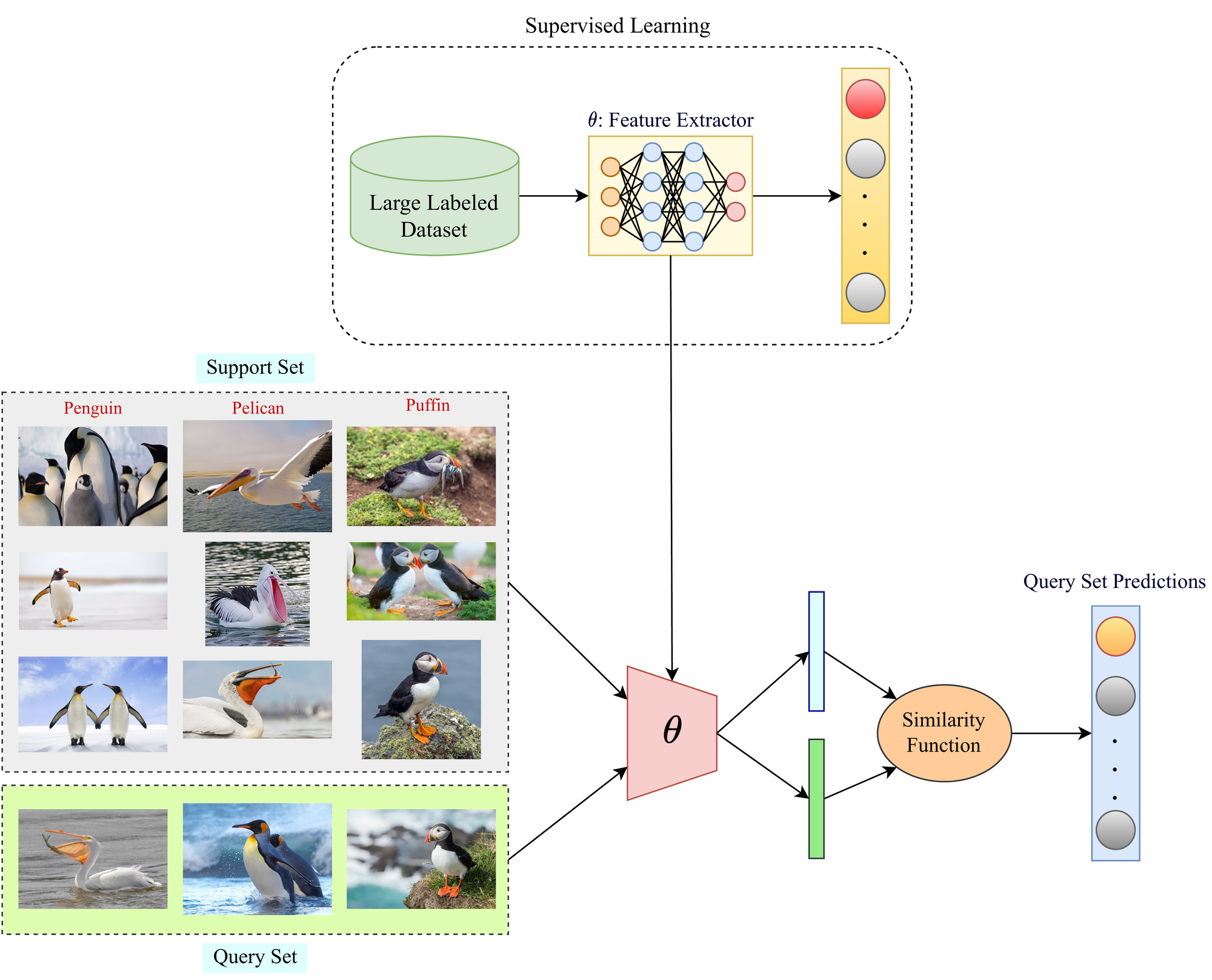
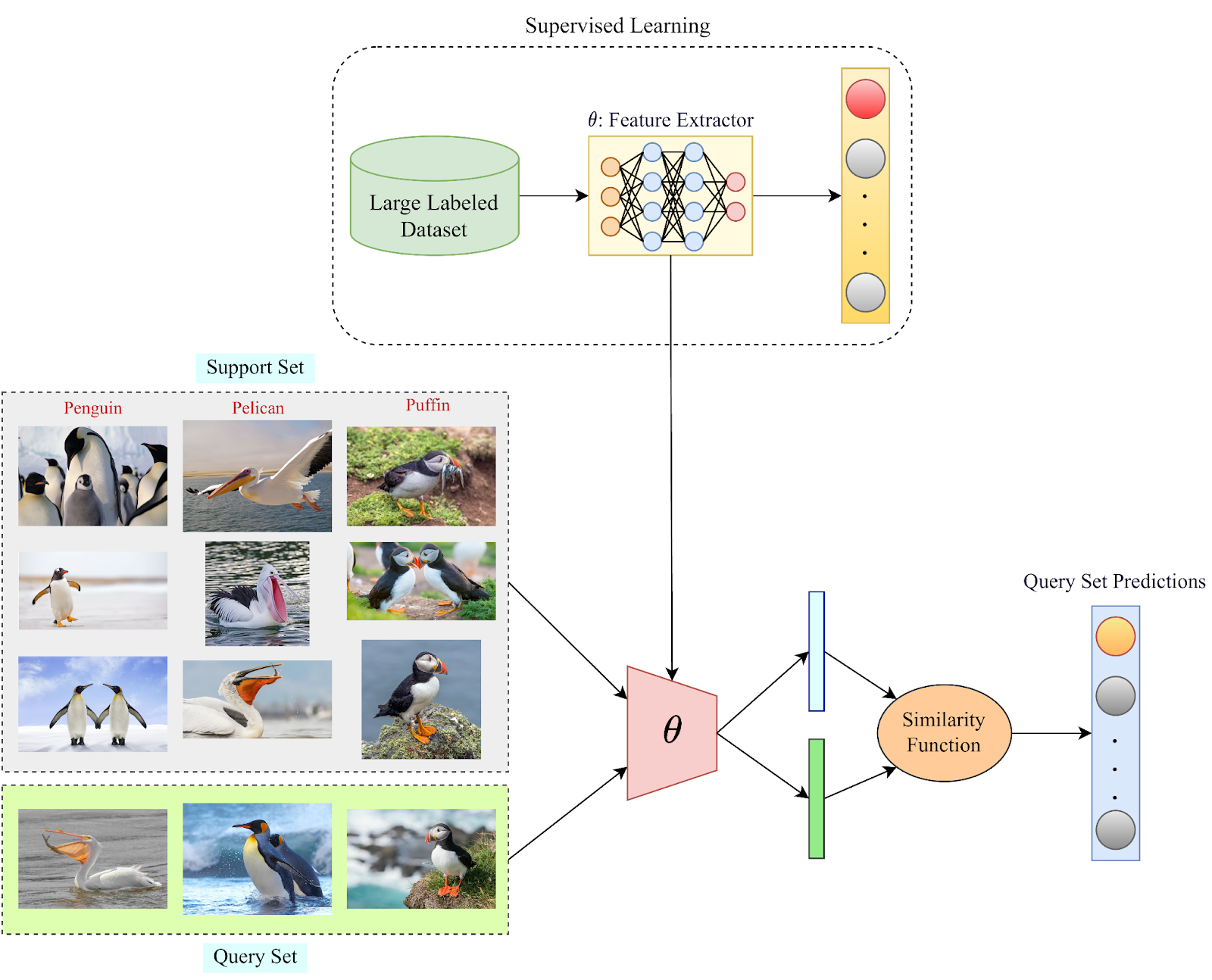
The primary goal in traditional Few-Shot frameworks is to learn a similarity function that can map the similarities between the classes in the support and query sets. Similarity functions typically output a probability value for the similarity.

For example, in the image below, a perfect similarity function should output a value of 1.0 when comparing two images of cats (I1 and I2). For the other two cases, where cat images are compared to an image of an ocelot, the similarity output should be 0.0. However, this is an ideal scenario. In reality, the values might be 0.95 for I1 and I2 and a small value greater than 0 for the other two cases (like 0.02 and 0.03).
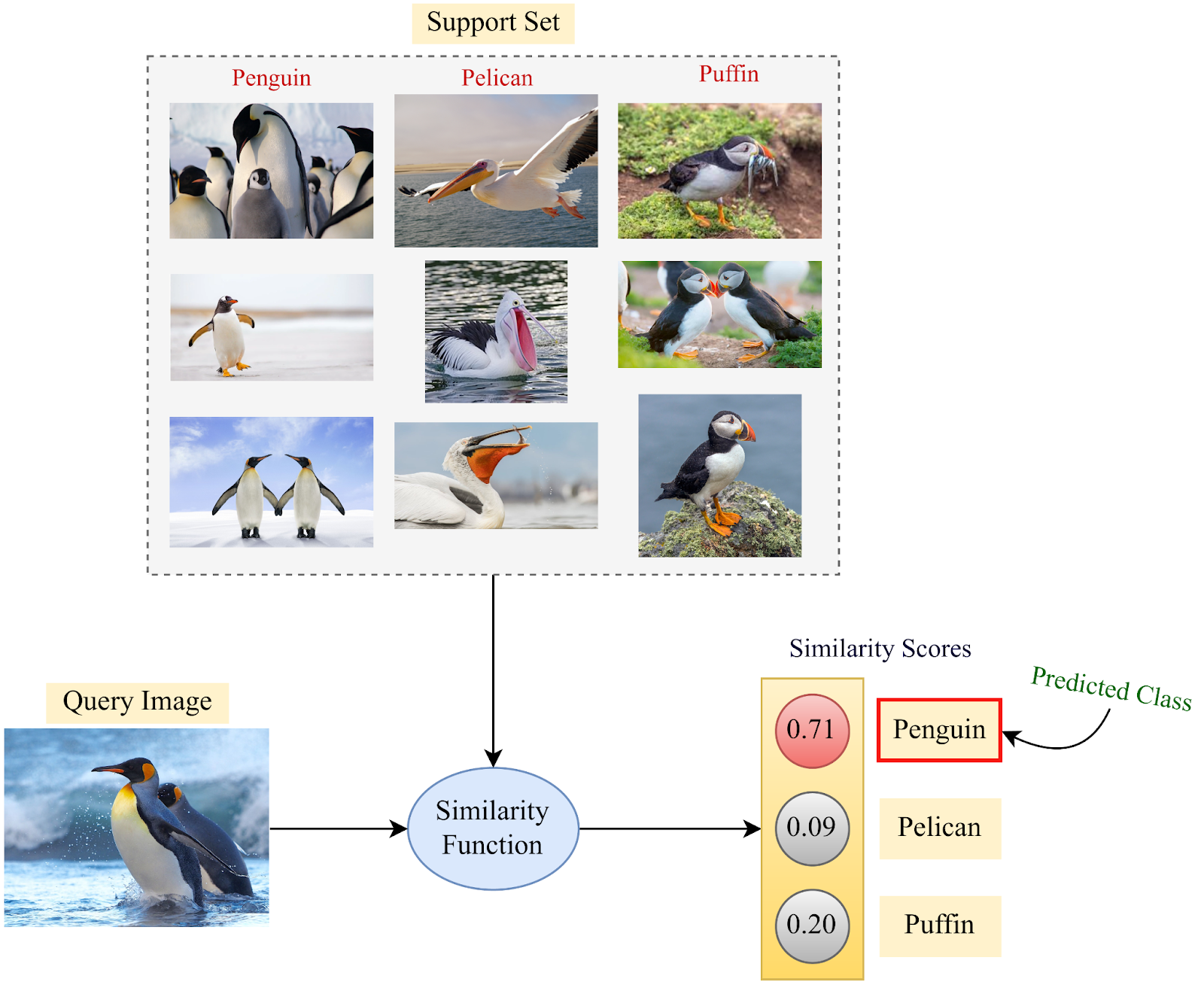
Now, we use a large-scale labeled dataset to train the parameters of such a similarity function. The training set used for pre-training the deep model in a supervised fashion can be used for this purpose. Once the parameters of the similarity function are trained, it can be used in the Few-Shot Learning phase for determining similarity probabilities on the query set by using the support set information. Then, for each query set sample, the class with the highest similarity from the support set will be inferred as the class label prediction by the Few-Shot model. One such example is illustrated above.
Siamese Network
In the Few-Shot Learning literature, similarity functions need not be “functions” at all. They can also, and will commonly, be neural networks: one of the most popular examples of which is the Siamese Network. The name is derived from the fact that “Siamese twins” are physically connected. Unlike traditional neural networks, which have one input branch and one output branch, a Siamese network has two or three input branches (based on the training method) and one output branch.
There are two ways to train a Siamese Network, which we will discuss next:
Method-1: Pairwise Similarity
In this method, a Siamese Network is given two inputs along with their corresponding labels (employing the training set used for the pre-trained feature extractor). Here, first, we select a sample from a dataset randomly (say, we choose the image of a dog). Then, we again choose a sample randomly from the dataset. If the second sample belongs to the same class as the first, that is, if the second image is again of a dog, then we assign a label of “1.0” as the ground truth for the Siamese Network. For all other classes, a label of “0.0” is assigned as the ground truth.

Thus, this network essentially learns a similarity matching criterion through labeled examples. This has been illustrated above using an example. Images are first passed through the same pre-trained feature extractor (typically, a Convolutional Neural Network) separately to obtain their corresponding representations. Then the two obtained representations are concatenated and passed through dense layers and a sigmoid activation function to obtain the similarity score. We already know whether the samples belong to the same class or not, so that information is used as the ground truth similarity score for calculating the loss and computing the back-propagation.
In Python3, the cosine similarity between two samples can be computed using the following:
import torch
import torch.nn as nn

input1 = torch.randn(100, 128)
input2 = torch.randn(100, 128)
cos = nn.CosineSimilarity(dim=1, eps=1e-6)
output = cos(input1, input2)
To get the images and the corresponding information about whether they belong to the same class or not, the following custom dataset needs to be implemented in Python3:
import random
from PIL import Image
import torchvision
import torchvision.datasets as datasets
import torchvision.transforms as transforms
from torch.utils.data import DataLoader, Dataset
import torchvision.utils
import torch
import torch.nn as nn

class SiameseDataset(Dataset):
    def __init__(self,folder,transform=None):
        self.folder = folder        #type: torchvision.datasets.ImageFolder
        self.transform = transform  #type: torchvision.transforms

    def __getitem__(self,index):
        #Random image set as anchor
        image0_tuple = random.choice(self.folder.imgs)

        random_val = random.randint(0,1)
        if random_val: #If random_val = 1, output a positive class sample
            while True:
                #Find "positive" Image
                image1_tuple = random.choice(self.folder.imgs)
                if image0_tuple[1] == image1_tuple[1]:
                    break
        else: #If random_val = 0, output a negative class sample
            while True:
                #Find "negative" Image
                image1_tuple = random.choice(self.folder.imgs)
                if image0_tuple[1] != image1_tuple[1]:
                    break

        image0 = Image.open(image0_tuple[0])
        image1 = Image.open(image1_tuple[0])

        image0 = image0.convert("L")
        image1 = image1.convert("L")

        if self.transform is not None:
            image0 = self.transform(image0)
            image1 = self.transform(image1)

        #Return the two images along with the information of whether they belong to the same class
        return image0, image1, int(random_val)

    def __len__(self):
        return len(self.folder.imgs)
Bring this project to life
Method-2: Triplet Loss
This method is based on a “triplet loss” criteria and can be thought of as an extension to Method-1, although the training strategy used here is different. First, we randomly choose a data sample from the dataset (training set), which we call the “anchor” sample. Next, we choose two other data samples- one from the same class as the anchor sample- called the “positive” sample, and another from a different class than the anchor- called the “negative” sample.
Once these three samples are selected, they are passed through the same neural network to obtain their corresponding representations in the embedding space. Then we calculate the L2 normalized distance between the anchor and the positive samples’ representations (let’s call it “d+”) and the L2 normalized distance between the anchor and the negative samples’ embedding (let’s call it “d-”). These parameters allow us to define a loss function that needs to be minimized, as illustrated below.

Here, “>0” is a margin that prevents the max function's two terms from being equal. The aim here is to push the representations of the anchor and negative samples as far as possible in the embedding space while pulling the representations for the anchor and negative samples as close as possible, as shown below.

Using PyTorch, Triplet Loss can be very easily implemented like the following (using an example of random anchor, positive and negative samples):
import torch
import torch.nn as nn

triplet_loss = nn.TripletMarginLoss(margin=1.0, p=2)
anchor = torch.randn(100, 128, requires_grad=True)
positive = torch.randn(100, 128, requires_grad=True)
negative = torch.randn(100, 128, requires_grad=True)
output = triplet_loss(anchor, positive, negative)
output.backward()
To generate anchor, positive and negative samples from an image dataset using PyTorch, the following custom dataset class needs to be written:
import random
from PIL import Image
import torchvision
import torchvision.datasets as datasets
import torchvision.transforms as transforms
from torch.utils.data import DataLoader, Dataset
import torchvision.utils
import torch
import torch.nn as nn

class SiameseDataset(Dataset):
    def __init__(self,folder,transform=None):
        self.folder = folder        #type: torchvision.datasets.ImageFolder
        self.transform = transform  #type: torchvision.transforms

    def __getitem__(self,index):
        #Random image set as anchor
        anchor_tuple = random.choice(self.folder.imgs)

        while True:
            #Find "positive" Image
            positive_tuple = random.choice(self.folder.imgs)
            if anchor_tuple[1] == positive_tuple[1]:
                break

        while True:
            #Find "negative" Image
            negative_tuple = random.choice(self.folder.imgs)
            if anchor_tuple[1] != negative_tuple[1]:
                break

        anchor = Image.open(anchor_tuple[0])
        positive = Image.open(positive_tuple[0])
        negative = Image.open(negative_tuple[0])

        anchor = anchor.convert("L")
        positive = positive.convert("L")
        negative = negative.convert("L")

        if self.transform is not None:
            anchor = self.transform(anchor)
            positive = self.transform(positive)
            negative = self.transform(negative)

        return anchor, positive, negative

    def __len__(self):
        return len(self.folder.imgs)
The above code can be implemented easily in Gradient. Simply open a Notebook with the advanced options "Workspace URL" field filled in with the following URL:
 gradient-ai
Approaches for Few-Shot Learning
Few-Shot Learning Approaches can be broadly classified into four categories which we shall discuss next:
Data-Level
Data-Level FSL approaches have a simple concept. If an FSL model training is stunted (and to prevent overfitting or underfitting) due to lack of training data, more data can be added - which may or may not be structured. That is, suppose we have two labeled samples per class in the support set, which may not be enough, so we can try augmenting the samples using various techniques.
Although data augmentation does not provide entirely new information per se, it can still be helpful for FSL training. Another method can be to add unlabeled data to the support set, making the FSL problem semi-supervised. The FSL model can use even the unstructured data to gather more information, which has proven to enhance few-shot performance.
Other methods also aim to use generative networks (like GAN models) to synthesize entirely new data from the existing data distribution. However, for GAN-based approaches, a lot of labeled training data is required to train the parameters of the model first before it can be used to generate new samples using a few support set samples.
Parameter-Level
In FSL, the availability of samples is limited; thus, overfitting is common since the samples have extensive and high-dimensional spaces. Parameter-level FSL approaches involve the use of meta-learning that control the exploitation of models’ parameters to intelligently infer which features are important for the task at hand.
FSL methods that constrain the parameter space and use regularization techniques fall under the category of parameter-level approaches. Models are trained to find the optimal route in the parameter space for providing targeted predictions.
Metric-Level
Metric-Level FSL approaches aim at learning a distance function between data points. Features are extracted from images, and the distance between the images is computed in the embedding space. This distance function can be Euclidean distance, Earth Mover Distance, Cosine Similarity-based distance, etc. This is something we have covered while discussing Siamese networks.
Such approaches enable the distance function to tune its parameters using the training set data that has been used to train the feature extractor model. Then, the distance function will draw inferences based on similarity scores (how close samples lie in the embedding space) between the support and query sets.
Gradient-based Meta-Learning
Gradient-based Meta-Learning approaches use two learners - a teacher model (base-learner) and a student model (meta-learner) using knowledge distillation. The teacher model guides the student model through the high-dimensional parameter space.
Using the information from the support set, the teacher model is first trained to make predictions on the query set samples. The classification loss derived from the teacher model is then used to train the student model, making it proficient in the classification task.
One-Shot Learning
As the discussion up to this point suggests, One-Shot Learning is a task where the support set consists of only one data sample per class. You can imagine that the task is more complicated with less supporting information. The face recognition technology used in modern smartphones uses One-Shot Learning.
One such example is the One-Shot Semantic Segmentation approach explored by Shaban et al. in this paper. The authors propose a novel two-branched approach, where the first branch takes the labeled image as input and produces a vector of parameters as output. The second branch takes these parameters as well as a new image as input and produces a segmentation mask of the image for the new class as output. Their architectural diagram is shown below.
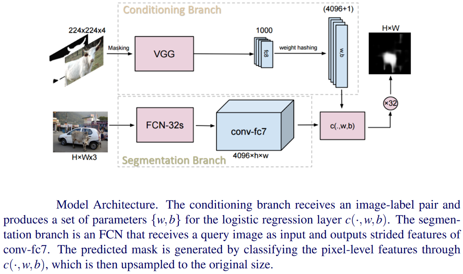
Unlike the fine-tuning approach to one-shot learning, which may require many iterations to learn parameters for the segmentation network, the first branch of this network computes parameters in a single forward pass. This has several advantages: 1) the single forward pass makes the proposed method fast; 2) the approach for one-shot learning is fully differentiable, allowing the branch to be jointly trained with the segmentation branch of the network; 3) finally, the number of parameters is independent of the size of the image, so the One-Shot method does not have problems in scaling.
Applications of Few-Shot Learning
Few-Shot Learning has been used extensively in several fields in the Deep Learning literature, from Computer Vision tasks like image classification and object detection to Remote Sensing, Natural Language Processing, etc. Let us briefly discuss them in this section.
Image Classification
Few-Shot Learning has been extensively used in image classification, some examples of which we have already explored.
Zhang et al., in their paper, proposed an interesting approach to Few-Shot Image Classification. A natural way to compare two complex structured representations is to compare their building blocks. The difficulty lies in that we do not have their correspondence supervision for training, and not all building elements can always find their counterparts in the other structures. To solve the problems above, the authors formalize the few-shot classification as an instance of optimal matching in this paper. The authors propose to use the optimal matching cost between two structures to represent their similarity.

Given the feature representations generated by two images, the authors adopt the Earth Mover’s Distance (EMD) to compute their structural similarity. EMD is the metric for computing distance between structural representations, originally proposed for image retrieval. Given the distance between all element pairs, EMD can acquire the optimal matching flows between two structures that have the minimum cost. It can also be interpreted as the minimum cost to reconstruct a structure representation with the other.
Object Detection
Object Detection is a computer vision problem of identifying and locating objects in an image or video sequence. A single image may contain a multitude of objects. So, it is different from simple image classification tasks where a whole image is given one class label.
This paper proposes the OpeN-ended Centre nEt (ONCE) model to address the problem of Incremental Few-Shot Detection Object Detection. The authors take a feature-based knowledge transfer strategy, decomposing a previous model called CentreNet into class-generic and class-specific components for enabling incremental few-shot learning. More specifically, ONCE first uses the abundant base class training data to train a class-generic feature extractor. This is followed by meta-learning, a class-specific code generator with simulated few-shot learning tasks. Once trained, given a handful of images of a novel object class, the meta-trained class code generator elegantly enables the ONCE detector to incrementally learn the novel class in an efficient feed-forward manner during the meta-testing stage (novel class registration).

Semantic Segmentation
Semantic Segmentation is a task where every pixel in an image is assigned a class- either one or more objects, or background. Few-Shot Learning has been used to perform binary and multi-label semantic segmentation in the literature.
Liu et al. proposed a novel prototype-based Semi-Supervised Few-Shot Semantic Segmentation framework in this paper, where the main idea is to enrich the prototype representations of semantic classes in two directions. First, they decompose the commonly used holistic prototype representation into a small set of part-aware prototypes, which is capable of capturing diverse and fine-grained object features and yields better spatial coverage in semantic object regions. Moreover, the authors incorporate a set of unlabeled images into their support set so that the part-aware prototypes can be learned from both labeled and unlabeled data sources. This enables them to go beyond the restricted small support set and to better model the intra-class variation in object features. The overview of their model is shown below.

Robotics
The field of robotics has also used Few-Shot Learning approaches to make robots mimic the ability of humans to generalize tasks using only a few demonstrations.
In an attempt to reduce the number of trials involved in learning, Wu et al. proposed an algorithm to address the “how-to” question in imitation in this paper. The authors introduce a novel computational model for learning path planning by imitation, which uses a fundamental idea in plan adaptation- the presence of invariant feature points in both the demonstration and a given situation- to generate a motion path for the new scenario.
Natural Language Processing
Few-Shot Learning has recently become popular in Natural Language Processing tasks as well, where labels for Language Processing are inherently difficult to come by.
For example, Yu et al. in their paper, tackle a text classification problem using Few-Shot Learning, specifically a metric-learning approach. Their meta-learner selects and combines multiple metrics for learning the target task using task clustering on the meta-training tasks. During the meta-training, the authors propose partitioning the meta-training tasks into clusters, making the tasks in each cluster likely to be related.

Then within each cluster, the authors train a deep embedding function as the metric. This ensures that the common metric is only shared across tasks within the same cluster. Further, during meta-testing, each target FSL task is assigned to a task-specific metric, which is a linear combination of the metrics defined by different clusters. In this way, the diverse few-shot tasks can derive different metrics from the previous learning experience.
Conclusion
Deep Learning has become a de-facto choice for solving complex Computer Vision and Pattern Recognition tasks. However, the need for large volumes of labeled training data and the computational cost incurred for training deep architectures hinder the progress of such tasks.
Few-Shot Learning is a workaround to this problem, allowing pre-trained deep models to be extended to novel data with only a few labeled examples and no re-training. Due to their reliable performance, tasks like image classification and segmentation, object recognition, Natural Language Processing, etc., have seen an uprising in the use of FSL architectures.
Research on better FSL models is still being actively pursued to make them as accurate or even better than fully-supervised learning approaches. Problems like One-Shot or Zero-Shot Learning which are significantly more complex, are being extensively studied to bridge the gap between AI and human learners.