Context Cluster: Image as Set of Points

Context Cluster

Convolutional Neural Networks and Vision based Transformer models (ViT) are widely spread techniques to process images and generate intelligent predictions. The ability of the model to generate predictions solely depends on the way it processes the image. CNNs consider an image as well-arranged pixels and extract local features using the convolution operation by filters in a sliding window fashion. On the other side, Vision Transformer (ViT) descended from NLP research and thus treats an image as a sequence of patches and will extract features from each of those patches. While CNNs and ViT are still very popular, it is important to think about other ways to process images that may give us other benefits.

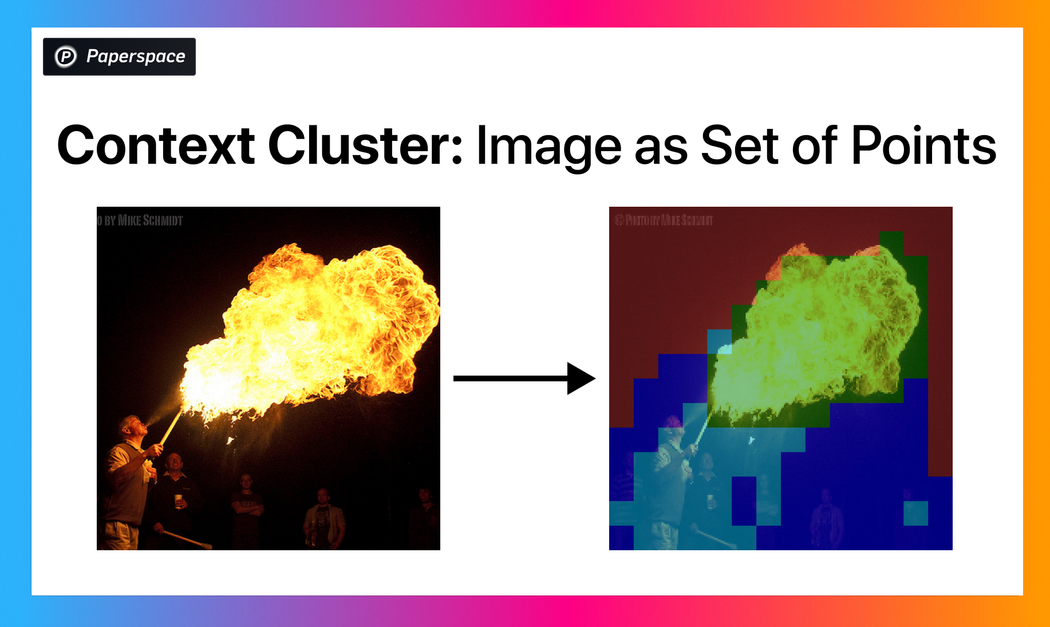
Researchers at Adobe & Northeastern University recently released a model named Context-Cluster. It treats an image as a set of many points. Rather than using sophisticated techniques, it utilizes the clustering technique to group these sets of points into multiple clusters. These clusters can be treated as groups of patches and can be processed differently for downstream tasks. We can utilize the same pixel embeddings for different tasks (classification, semantic segmentation, etc.)

Model architecture

Initially, we have an image of shape (3, W, H) denoting the number of channels, width, and height of the image. This raw image contains 3 channels (RGB) representing different color values. To add 2 more data points, we also consider the position of the pixel in the W x H plane. To enhance the distribution of the position feature, the position value (i, j) is converted to (i/W - 0.5, j/H - 0.5) for all pixels in an image. Eventually, we end up with the dataset with shape (5, N) where N represents the number of pixels (W * H) in the image. This type of representation of image can be considered universal since we haven't assumed anything until now.

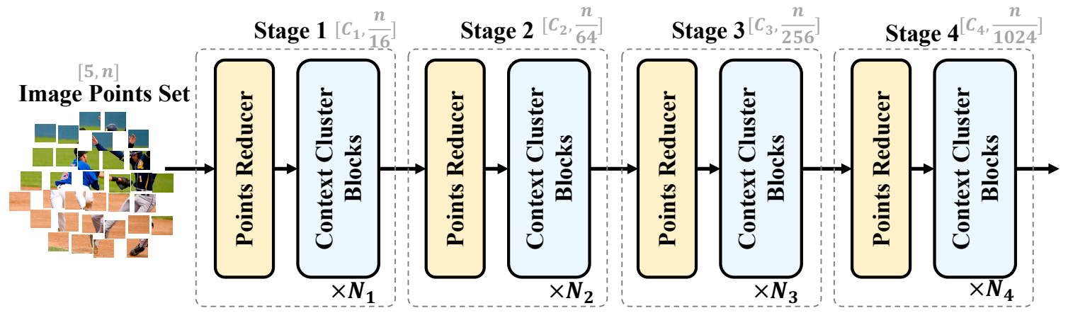
Now if we recall the traditional clustering methodology (K-means), we need to assign some random points as cluster centers and then compute the nearest cluster center for all the available data points (pixels). But since the image can have arbitrarily large resolution and thus will have too many pixels of multiple dimensions in it. Computing the nearest cluster center for all of them will not be computationally feasible. To overcome this issue, we first reduce the dimension of points for the dataset by an operation called Point Reducer. It reduces the dimension of the points by linearly projecting (using a fully connected layer) the dataset. As a result, we get a dataset of dimension (N, D) where D is the number of features of each pixel.

The next step is context clustering. It randomly selects some c center points over the dataset, selects k nearest neighbors for each center point, concatenates those k points, and inputs them to the fully connected linear layer. Outputs of this linear layer are the features for each center point. From the c-center features, we define the pairwise cosign similarity of each center with each pixel. The shape of this similarity matrix is (C, N). Note here that each pixel is assigned to only a single cluster. It means it is hard clustering.

Now, the points in each cluster are aggregated based on the similarity to the center. This aggregation is done similarly using a fully connected layer(s) and converts features of M data points within the cluster to shape (M, D'). This step applies to the points in each cluster independently.  It aggregates features of all the points within the cluster. Think of it like the points within each cluster sharing information. After aggregation, the points are dispatched back to their original dimension. It is again performed using a fully connected layer(s). Each point is again transformed back into D dimensional feature.

The described 4 steps (Point Reducer, Context Clustering, Feature Aggregation & Feature Dispatching) create a single stage of the model. Depending on the complexity of the data, we can add multiple such stages with different reducing dimensions so that it improves its learning directions. The original paper describes a model with 4 stages as shown in Fig 1.

After computing the last stage of the model, we can treat the resultant features of each pixel differently depending on the downstream task. For the classification task, we can calculate the average of all the point features and pass it through fully connected layer(s) which is attached to softmax or sigmoid function to classify the logits. For the dense prediction task like segmentation, we need to position the data points by their location features at the end of all stage computation. As part of this blog, we will perform a cluster visualization task that is somewhat similar to a segmentation task.

Comparison with other models

The context cluster model is trained in different variants: tiny, small & medium. The variant mostly has differences in depth (number of stages). The context cluster model is trained for 310 epochs on the ImageNet dataset. It is then compared to other popular models which use Convolutional Neural Networks (CNNs) and Transformers. The model is trained and compared for several tasks like image classification, object detection, 3D point cloud classification, semantic segmentation, etc. The models are compared for different metrics like the number of parameters, number of FLOPs, top-1% accuracy, throughputs, etc.

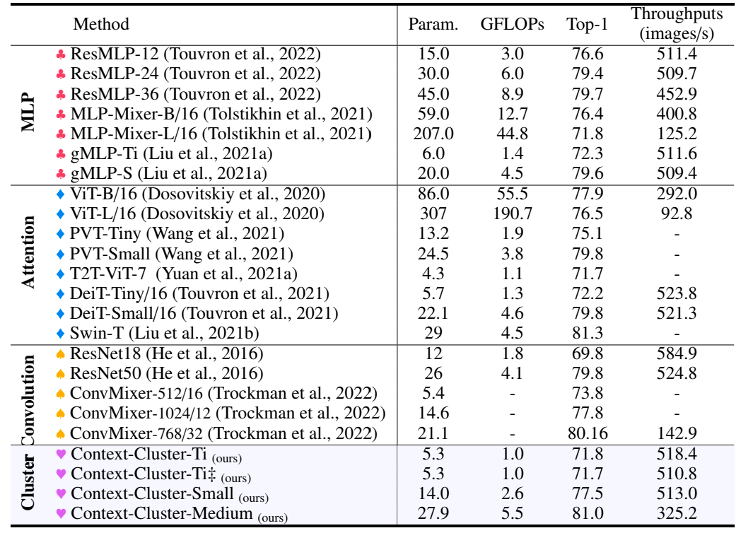
Fig. 2 shows the comparison of different variants of context-cluster models with many other popular computer vision models. The above-shown comparison is for the classification task. The paper also has similar comparison tables for other tasks which you might be interested in looking at.  

We can notice in the comparison table that the context cluster models have comparable & sometimes better accuracy as compared to other models. It also has a lesser number of parameters and FLOPs than many other models. In use cases where we have huge data of images to classify and we can bear little accuracy loss, context cluster models might be a better choice.

Try it yourself

Let us now walk through how you can download the dataset & train your own context cluster model. For the demo purpose, you don't need to train the model. Instead, you can download pre-trained model checkpoints to try. For this task, we will get this running in a Gradient Notebook here on Paperspace. To navigate to the codebase, click on the "Run on Gradient" button above or at the top of this blog.

Setup

The file installations.sh contains all the necessary code to install the required things. Note that your system must have CUDA to train Context-Cluster models. Also, you may require a different version of  torch based on the version of CUDA. If you are running this on Paperspace, then the default version of CUDA is 11.6 which is compatible with this code. If you are running it somewhere else, please check your CUDA version using nvcc --version. If the version differs from ours, you may want to change versions of PyTorch libraries in the first line of installations.sh by looking at compatibility table.

To install all the dependencies, run the below command:

bash installations.sh

The above command also clones the original Context-Cluster repository into context_cluster directory so that we can utilize the original model implementation for training & inference.

Downloading datasets & Start training (Optional)

Once we have installed all the dependencies, we can download the datasets and start training the models.

dataset directory in this repo contains the necessary scripts to download the data and make it ready for training. Currently, this repository supports downloading ImageNet dataset that the original authors used.

We have already setup bash scripts for you which will automatically download the dataset for you and will start the training. train.sh contains the code which will download the training & validation data to dataset the directory and will start training the model.

This bash script is compatible to the Paperspace workspace. But if you are running it elsewhere, then you will need to replace the base path of the paths mentioned in this script train.sh.

Before you start the training, you can check & customize all the model arguments in args.yaml file. Especially, you may want to change the argument model to one of the following: coc_tiny, coc_tiny_plain, coc_small, coc_medium. These models differ by the number of stages.

To download data files and start training, you can execute the below command:

bash train.sh

Note that the generated checkpoints for the trained model will be available in context_cluster/outputs directory. You will need to move checkpoint.pth.tar file to checkpoints directory for inference at the end of training.

Don't worry if you don't want to train the model. The below section illustrates downloading the pre-trained checkpoints for inference.

Running Gradio Demo

Python script app.py contains Gradio demo which lets you visualize clusters on the image. But before we do that, we need to download the pre-trained checkpoints into checkpoints directory.

To download existing checkpoints, run the below command:

bash checkpoints/fetch_pretrained_checkpoints.sh

Note that the latest version of the code only has the pre-trained checkpoints for coc_tiny_plain  model variant. But you can add the code in checkpoints/fetch_pretrained_checkpoints.sh whenever the new checkpoints for other model types are available in original repository.

Now, we are ready to launch the Gradio demo. Run the following command to launch the demo:

gradio app.py

Open the link provided by the Gradio app in the browser and now you can generate inferences from any of the available models in checkpoints directory. Moreover, you can generate cluster visualization of specific stage, block and head for any image. Upload your image and hit the Submit button.

You should be able to generate cluster visualization for any image as shown below:

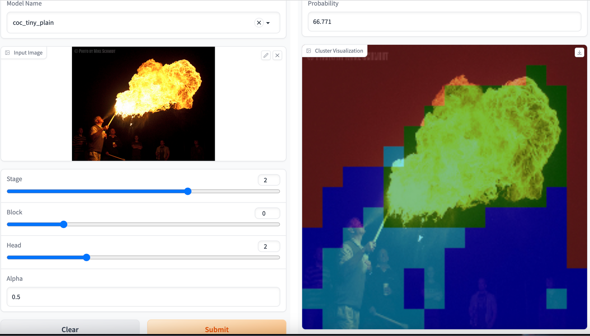
Hurray! 🎉🎉🎉 We have created a demo to visualize clusters over any image by inferring the Context-Cluster model.

Conclusion

Context-Cluster is a computer vision technique that treats an image as a set of points. It is very different from how CNNs and Vision based Transformer models process images. By reducing the points, the context cluster model performs intelligent clustering over the image pixels and partitions images into different clusters. It has a comparatively lesser number of parameters and FLOPs. In this blog, we walked through the objective & the architecture of the Context-Cluster model, compared the results obtained from Context-Cluster with other state-of-the-art models, and discussed how to set up the environment, train your own Context-Cluster model & generate inference using Gradio app on Gradient Notebook.

Be sure to try out each of the model varieties using Gradient's wide range of available machine types!