Fine-Tuning Shallow Networks with Keras for Efficient Image Classification

Neural networks with extensively deep architectures typically contain millions of parameters, making them both computationally expensive and time-consuming to train. In this tutorial, we'll achieve state-of-the-art image classification performance using DenseNet, initially with a single hidden layer. For this study, we systematically tuned the number of neurons in the hidden layer and trained our model on a benchmark image classification dataset. This study shows that building deeper neural networks is not always necessary; instead, it is more important to focus on the correct number of neurons in each layer.

You can follow along with the code and run it for free from the ML Showcase.

Introduction

In 2012, Krizhevsky et al. introduced AlexNet for image classification $[1]$, which has overall 660,000 neurons, 61 million parameters, and 600 million connections. It took the authors six days to train their network on two Nvidia Geforce GTX 580 GPUs in parallel over 90 epochs. Later, in 2014, VGG-16 was introduced by Simonyan et al. $[2]$. It contained 138M parameters collectively. From then on it has become a trend to design more and more complex neural network structures, incorporating a significant number of parameters.

Motivation

Creating deeper neural networks requires more sophisticated hardware, such as high GPU memory, which can be expensive. Training a network for days or weeks is also not always an option. In this study we tuned the number of neurons, the different activation functions, dropout rates, and having only one layer, attempted to gain AlexNet-level accuracy. We performed experimentation on the Fashion-MNIST benchmark dataset introduced by Xiao et al. $[3]$.

Objective

Our main objective in this experiment is to determine the optimal neural network architectures with as few parameters as possible, while not compromising the performance. Additionally, this work also exposes the capability of hidden layers with an optimal number of neurons. Moreover, we tried our best to keep our approach as simple as possible without fancy stages, such as image augmentation, image up-scaling, or others. Standard AlexNet requires 256×256 RGB images, yet we applied 28×28 grayscale images and compared performances to have a proper glimpse of shallow network stability on a low-quality dataset. This study is especially important to improve performance on low-memory resources, as even a 256×256 grayscale image dataset would require significant memory.

Dataset

The Fashion-MNIST dataset contains 60,000 training and 10,000 testing 28×28 pixel grayscale images across 10 classes $[3]$. As reported by Ma et al., the accuracy performance of AlexNet on the Fashion-MNIST dataset is 86.43% $[4]$.

A note regarding the AlexNet input (from here):

The input to AlexNet is an RGB image of size 256×256. This means all images in the training set and all test images need to be of size 256×256.

If the input image is not 256×256, it needs to be converted to 256×256 before using it for training the network. To achieve this, the smaller dimension is resized to 256 and then the resulting image is cropped to obtain a 256×256 image.
...
If the input image is grayscale, it is converted to an RGB image by replicating the single channel to obtain a 3-channel RGB image.

We will present the corresponding code snippets in this article for each step. We have used Keras for implementation purposes. Note that you can run the code for free on Gradient.

Import Dataset

import keras

(x_train, y_train), (x_test, y_test) = keras.datasets.fashion_mnist.load_data()

print('x_train.shape =',x_train.shape)
print('y_train.shape =',y_train.shape)
print('x_test.shape =',x_test.shape)
print('y_test.shape =',y_test.shape)

Expected output:

x_train.shape = (60000, 28, 28)
y_train.shape = (60000,)
x_test.shape = (10000, 28, 28)
y_test.shape = (10000,)

Get the number of classes in the dataset

import numpy as np

num_classes = np.unique(y_test).shape[0]
print('num_classes =', num_classes)

Expected output:

num_classes = 10

Data Preparation

Normalize values in each image matrix within range $[0,1]$ in the dataset:

x_train_norm = x_train/255
x_test_norm = x_test/255

Dense networks expect input shape as (batch_size, width, height, channel). Hence, expand dimensions of the training and test data sets:

final_train_imageset = np.expand_dims(x_train_norm, axis = 3)
final_test_imageset = np.expand_dims(x_test_norm, axis = 3)

y_train2 = np.expand_dims(y_train, axis = 1)
y_test2 = np.expand_dims(y_test, axis = 1)

print('final_train_imageset.shape =', final_train_imageset.shape)
print('final_test_imageset.shape =', final_test_imageset.shape)
print('y_train2.shape =', y_train2.shape)
print('y_test2.shape =', y_test2.shape)

Expected output:

final_train_imageset.shape = (60000, 28, 28, 1)
final_test_imageset.shape = (10000, 28, 28, 1)
y_train2.shape = (60000, 1)
y_test2.shape = (10000, 1)

In order to use categorical_crossentropy as the loss function, we have to apply one-hot encoding to the labels.

final_train_label = keras.utils.to_categorical(y_train2, num_classes)
final_test_label = keras.utils.to_categorical(y_test2, num_classes)

print('final_train_label.shape =',final_train_label.shape)
print('final_test_label.shape =',final_test_label.shape)

Expected output:

final_train_label.shape = (60000, 10)
final_test_label.shape = (10000, 10)

Generic DenseNet Structure

We first experimented thoroughly with only a single hidden layer. Later in this article we add another hidden layer to two of the best-performing single-layer architectures.

Single-Layer DenseNet

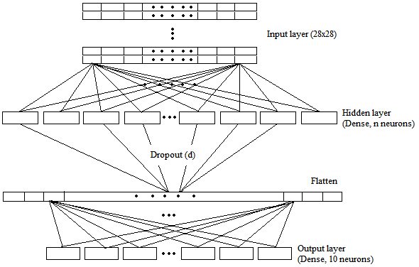
We have visualized the generic DenseNet structure with a single hidden layer in Figure 1. It contains three layers: an input layer, a hidden layer, and an output layer. In the input layer, 28×28 pixel images are provided to the network. The output layer has ten neurons corresponding to ten classes. We tuned the number of neurons in the hidden layer based on the number of total pixels in an image. An image has 28×28 (784) pixels. We started training our model with the number of neurons (n) equivalent to 1% of the total number of pixels, that is, seven neurons only (784×0.01). Then, we gradually increased neurons by taking 78 (10%), 392 (50%), and 784 (100%) neurons. Outputs from the hidden layer were flattened before the output layer.

Setting up necessary parameters and variables:

percentile = 1.0 # 1.0, 0.5, 0.1, 0.01

NUM_NEURONS = (x_train.shape[1]*x_train.shape[2])*percentile
NUM_LAYERS = 1
BATCH_SIZE = 128
NUM_EPOCHS = 3000
LEARNING_RATE = 0.0001
EPSILON = 1e-4
DROPOUT = 0.5 # 0.5, 0.8

LOSS = 'categorical_crossentropy'
DENSE_ACTIVATION_FUNCTION = 'default' # default, relu, LeakyReLU, PReLU, ELU
FINAL_ACTIVATION_FUNCTION = 'softmax'
early_stop_after_epochs = 50 # stop after 50 consecutive epochs with no improvement
validation_split = 0.1

checkpointer_name = "weights.Dense.Fashion.nLayers"+str(NUM_LAYERS)+".nNeurons"+str(NUM_NEURONS)+".act."+DENSE_ACTIVATION_FUNCTION+".p"+str(percentile)+".dropout"+str(DROPOUT)+".batch"+str(BATCH_SIZE)+".hdf5"

In general we used 50% dropout (d) for the hidden layer. However, in two cases we applied an 80% dropout to reduce overfitting. Each hidden unit was tested without any activation function, and with a ReLU activation. In the final layer, we applied softmax activation as the classifier. Moreover, in all cases we initialized biases with zeros and employed glorot_uniform as the kernel initializer. It helps the network to converge faster to the optimal solution. All the tasks were implemented with the Keras Function API.

Make a choice-list of activation functions:

def dense_activation():
    if DENSE_ACTIVATION_FUNCTION == 'relu':
        keras.layers.ReLU(max_value=None, negative_slope=0, threshold=0)
    elif DENSE_ACTIVATION_FUNCTION == 'LeakyReLU':
        keras.layers.LeakyReLU(alpha=0.3)
    elif DENSE_ACTIVATION_FUNCTION == 'PReLU':
        keras.layers.PReLU(tf.initializers.constant(0.3)) # "zeros"
    elif DENSE_ACTIVATION_FUNCTION == 'ELU':
        keras.layers.ELU(alpha=1.0)
    elif DENSE_ACTIVATION_FUNCTION == 'default':
        return None

The total number of trainable parameters were around 54K, 611K, 3M, and 6.1M for the corresponding 7, 78, 392, and 784 neurons in the hidden layer. There were no non-trainable parameters. We took 10% of the training data for validation and continued training each model until there were 50 consecutive epochs without improvement in validation loss.

Code for the model:

from keras.layers import *
from keras.models import * #Model, load_model

input_shape = final_train_imageset.shape[1:]

# Input tensor shape
inputs = Input(input_shape)

x = inputs
for _ in range(NUM_LAYERS):
    x = Dense(NUM_NEURONS, activation=dense_activation())(x)
    x = Dropout(DROPOUT)(x)

x = Flatten()(x)
outputs = Dense(num_classes, activation=FINAL_ACTIVATION_FUNCTION)(x)

model = Model(inputs=inputs, outputs=outputs)
model.summary()

The structure should be the following:

Model: "functional_9"
_________________________________________________________________
Layer (type)                 Output Shape              Param #   
=================================================================
input_6 (InputLayer)         [(None, 28, 28, 1)]       0         
_________________________________________________________________
dense_8 (Dense)              (None, 28, 28, 784)       1568      
_________________________________________________________________
dropout_4 (Dropout)          (None, 28, 28, 784)       0         
_________________________________________________________________
flatten_4 (Flatten)          (None, 614656)            0         
_________________________________________________________________
dense_9 (Dense)              (None, 10)                6146570   
=================================================================
Total params: 6,148,138
Trainable params: 6,148,138
Non-trainable params: 0
_________________________________________________________________

Define some widely used optimizers:

optimizer_1 = keras.optimizers.RMSprop(lr = LEARNING_RATE, epsilon=EPSILON)
optimizer_2 = keras.optimizers.Adam(lr = LEARNING_RATE, epsilon=EPSILON, beta_1=0.9, beta_2=0.999, amsgrad=False)
optimizer_3 = keras.optimizers.SGD(lr = LEARNING_RATE, momentum=0.85)

Let's choose Adam optimizer and compile the model:

model.compile(
    optimizer=optimizer_2, # 'Adam'
    loss=LOSS,
    metrics=['accuracy', 'Precision', 'Recall']
)

Set model checkpointer:

from tensorflow.keras.callbacks import EarlyStopping, ModelCheckpoint

checkpointer_best = ModelCheckpoint(filepath = checkpointer_name, 
                                    monitor='val_loss', 
                                    save_weights_only=False,
                                    mode='auto',  
                                    verbose = 2, 
                                    save_best_only = True
                                    )
                                    
early_stopping = EarlyStopping(monitor='val_loss', patience=early_stop_after_epochs)

Train the model:

list_callbacks = [checkpointer_best, early_stopping]

history = model.fit(final_train_imageset, final_train_label, 
                        shuffle=True, 
                        batch_size = BATCH_SIZE, 
                        epochs = NUM_EPOCHS,
                        validation_split = validation_split,
                        callbacks=list_callbacks
                    )

Performance Evaluation for Single-Layer DenseNet

Now, load the trained model and evaluate using the test set:

model_loaded = load_model(checkpointer_name)
result = model_loaded.evaluate(final_test_imageset, final_test_label)

We have summarized our experimental results in Table 1 (below).

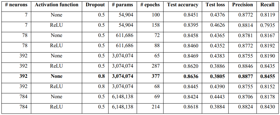
As the highest test accuracy (86.20%) with lowest test loss (0.39) in the single-layer models was achieved with 392 neurons (with ReLU activation), we trained the models with 392 neurons with 80% dropout both with and without activation. A point to be noted is that the second-best model in terms of test accuracy was also with 392 neurons; however, without activation (84.69%).

Finally, for 392 hidden neurons with 80% dropout, the respective test accuracy, test loss, Precision, and Recall were 86.36%, 0.38, 88.77%, and 84.55%, over 377 epochs without activation. However, with ReLU activation, the corresponding results were 84.45%, 0.44, 87.55%, and 81.52% over only 68 epochs.

Overall, the best performance was achieved by the model consisting of 392 hidden units with an 80% dropout without any activation function. The performance (86.36% test accuracy) was almost the same as the accuracy level of AlexNet (86.43%).

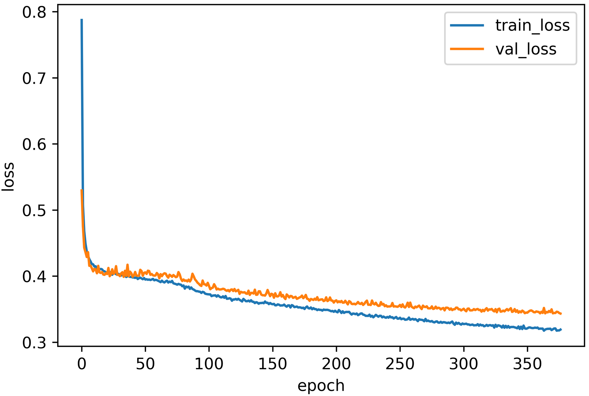
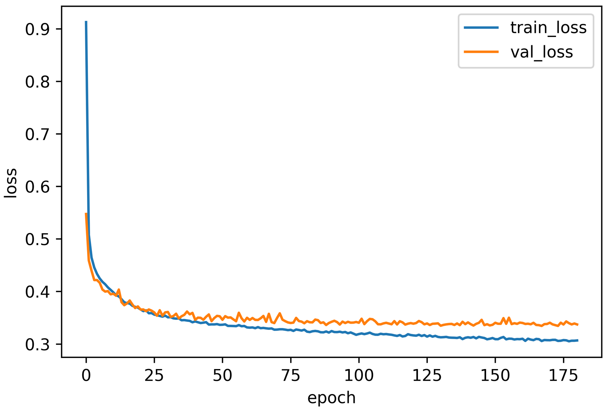
Let's plot the learning curve:

import matplotlib.pyplot as plt

plt.plot(history.history['loss'])
plt.plot(history.history['val_loss'])
plt.title(title)
plt.ylabel('loss')
plt.xlabel('epoch')
plt.legend(['train_loss','val_loss'], loc = 'best')

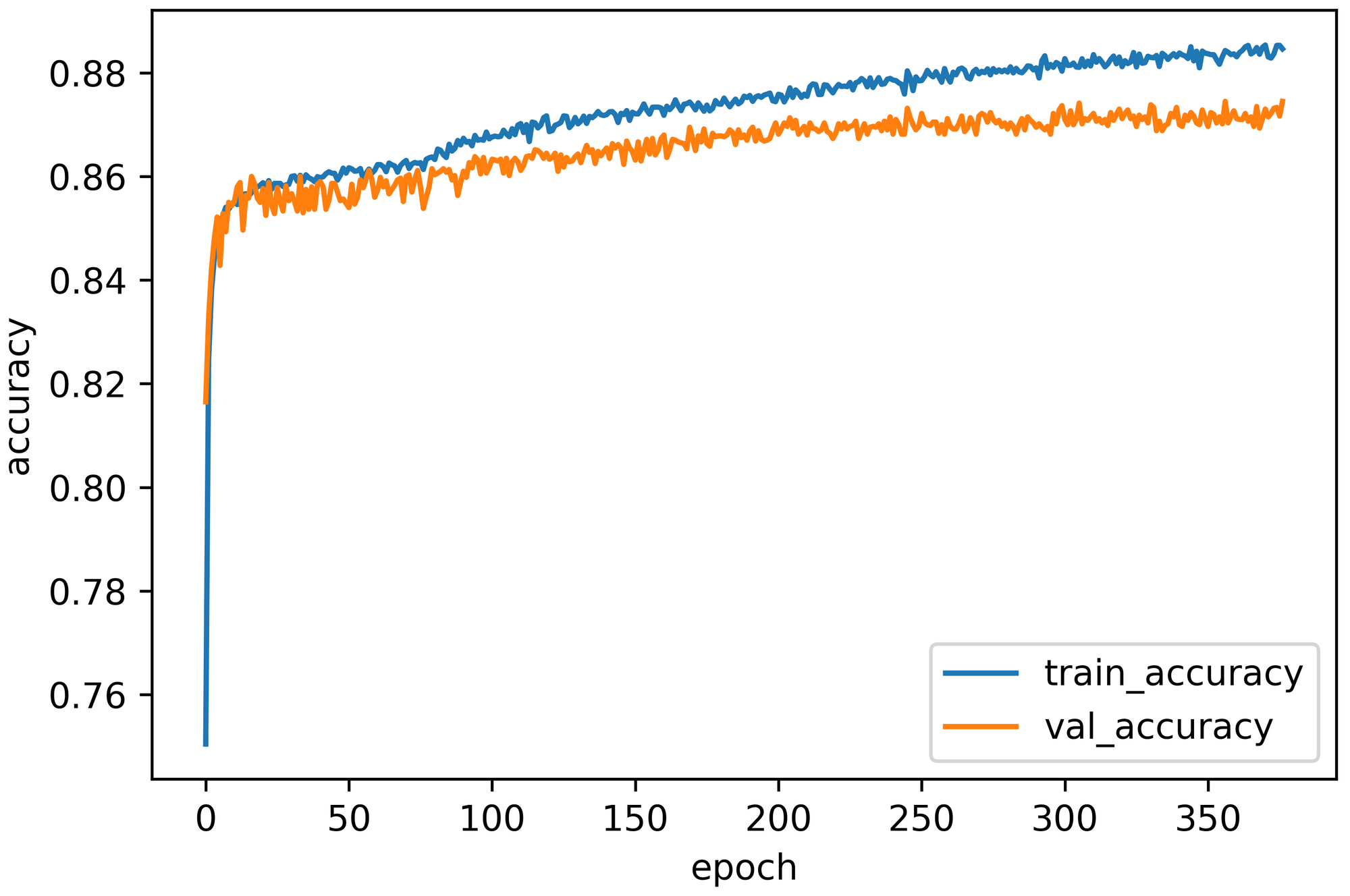
Also, visualize the training and validation accuracy trends while training:

plt.plot(history.history['accuracy'])
plt.plot(history.history['val_accuracy'])
plt.title(title)
plt.ylabel('accuracy')
plt.xlabel('epoch')
plt.legend(['train_accuracy','val_accuracy'], loc = 'best')

Multi-Layer DenseNet

Now that we have experimented with tuning the number of neurons in a network with a single hidden layer, let's add another hidden layer. Here we have examined two different networks with double hidden layers. The first one contains 78 neurons, and the second one contains 392 neurons in each hidden layer.

Performance Evaluation for Multi-Layer DenseNet

For the first architecture, the test loss, test accuracy, Precision, and Recall were 0.3691, 86.71%, 89%, and 84.72%, respectively. Figure 4 represents the training versus validation curves for this network.

Contrarily, the second network architecture's performance was 0.3721, 86.66%, 88.87%, and 84.91%, accordingly. Figure 5 demonstrates the learning curve (validation loss) in contrast to the training loss curve.

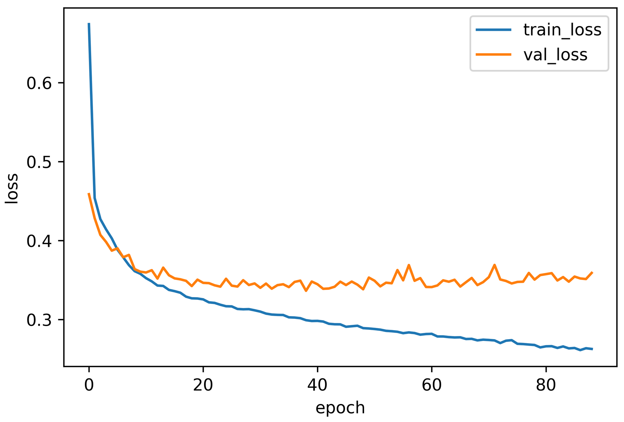
Notice that while several implementations in a single hidden layer achieved almost AlexNet-level accuracy, both implementations with a double hidden layer overcame AlexNet performance. Additionally, adding more neurons does not always lead to better results and can make the neural network more vulnerable to over-fitting.

Suggestions for Future Contributions

In this work we experienced the powerful capability of the hidden neurons in shallow networks to learn data. We compared the single and double hidden-layer models with the deeper AlexNet architecture. Nonetheless, these results should be further investigated intensely with other benchmark datasets. Also, we can examine if these behaviors are applicable to images with much lower dimensions. We should additionally construct a similar type of shallow convolutional model to observe the effects. Considering an optimal number of neurons with the correct configuration, we hope that this type of shallow model would largely eradicate our necessity for heavyweight models, thus reducing expensive hardware requirements and time complexity.

References

1. Krizhevsky, A., Sutskever, I., & Hinton, G. E. (2012). Imagenet classification with deep convolutional neural networks. In Advances in neural information processing systems (pp. 1097-1105).
2. Simonyan, K., & Zisserman, A. (2014). Very deep convolutional networks for large-scale image recognition. arXiv preprint arXiv:1409.1556.
3. Xiao, H., Rasul, K., & Vollgraf, R. (2017). Fashion-mnist: a novel image dataset for benchmarking machine learning algorithms. arXiv preprint arXiv:1708.07747.
4. Ma, B., Li, X., Xia, Y., & Zhang, Y. (2020). Autonomous deep learning: A genetic DCNN designer for image classification. Neurocomputing, 379, 152-161.