Bring this project to life
Introduction
PyTorch libraries like Torchvision and Torchtext support specialized data such as computer vision and natural language data. The torchvision.datasets module demonstrates how to load data using built-in classes. When using the torchvision.datasets module, you can load image data from well-known datasets through various subclasses. This tutorial demonstrates how to apply model interpretability algorithms from Captum library on a simple model and test samples from CIFAR dataset.
In this tutorial, we will build a basic model similar to the one presented here. Then, we will use attribution algorithms such as IntegratedGradients, Saliency, DeepLift and NoiseTunnel to attribute the label of the image to the input pixels and visualize it. Installing the torchvision and captum is required before following this tutorial.
Import the Libraries:
import matplotlib.pyplot as plt
import numpy as np

%matplotlib inline

import torch
import torchvision
import torchvision.transforms as transforms
import torchvision.transforms.functional as TF
import torch.optim as optim
import torch.nn as nn
import torch.nn.functional as F

from torchvision import models

from captum.attr import IntegratedGradients
from captum.attr import Saliency
from captum.attr import DeepLift
from captum.attr import NoiseTunnel
from captum.attr import visualization as v
Preparing your Data for Training with DataLoaders
We load the test and train datasets through the code below, define image transformers, and support classification label classes. Before the data is used for training and testing with the NN model, some adjustments may need to be made to the data. The data's values can be normalized to facilitate the training process, supplemented to produce more extensive datasets, or changed from one type of object to a tensor.
Through the use of the transforms.compose, we define a collection of transforms. This class will take a list of transformations and then apply them in the order given. In this step, we first convert images to tensors and then normalize the values of the tensors according to preset means and standard deviations. The torch.utils.data.DataLoader class makes it simple to proceed with batch processing.
It is a common practice to feed samples through a model in "mini batches," reshuffle data at each iteration to minimize overfitting, and leverage Python's multiprocessing to speed up data retrieval. An iterable called a DataLoader wraps this complexity for us in a straightforward API. Our model uses two convolutional layers, two max-pooling layers, and three fully connected or linear layers.
class Net(nn.Module): ## create layers as class attributes
    def __init__(self): ## Parameters initialization with __init__() function
        super(Net, self).__init__() ## call the parent constuctor
        self.conv1 = nn.Conv2d(3, 6, 5) ## Appy our first set of conv layers
        self.pool1 = nn.MaxPool2d(2, 2) ## Apply our first set of max pooling layers
        self.pool2 = nn.MaxPool2d(2, 2) ## Apply our second set of maxpooling layers
        self.conv2 = nn.Conv2d(6, 16, 5) ## second set of conv layers
        self.fc1 = nn.Linear(16 * 5 * 5, 120) ##first set of fully conneted layers
        self.fc2 = nn.Linear(120, 84) ## second set of fullly conneted layers
        self.fc3 = nn.Linear(84, 10) ## third set of fully connected layer
        self.relu1 = nn.ReLU() ## Apply RELU activation function
        self.relu2 = nn.ReLU()
        self.relu3 = nn.ReLU()
        self.relu4 = nn.ReLU()

    def forward(self, x): ## specify how the model handles the data.
        x = self.pool1(self.relu1(self.conv1(x)))
        x = self.pool2(self.relu2(self.conv2(x)))
        x = x.view(-1, 16 * 5 * 5)
        x = self.relu3(self.fc1(x))
        x = self.relu4(self.fc2(x))
        x = self.fc3(x)
        return x

## Model initialization
net = Net()
Define Loss Function and Optimizer
Next, we need to specify the loss function (also known as the criterion), and the technique for optimizing it. The loss function determines how well our model performs, which is used to compute the loss between actual results and forecasts. During training, we'll tweak the model parameters to minimize the loss. Ensure to include the model.parameters() for your model in the code. This tutorial uses the CrossEntropyLoss() function in conjunction with the stochastic gradient descent (SGD) optimizer. The following code shows how to use the torch.optim and torch.nn packages to create a loss function and an optimizer.
# Initialize criterion and optimizer
criterion = nn.CrossEntropyLoss()
optimizer = optim.SGD(net.parameters(), lr=0.001, momentum=0.9)
Train the Model
We keep a version of the pre-trained model in the 'models' folder so that we can load it without having to start the training process from the very beginning each time. You can download it here:
https://github.com/pytorch/captum/blob/master/tutorials/models/cifar_torchvision.pt
USE_PRETRAINED_MODEL = True
## If using the pretrained model, load it through the function load_state_dict
if USE_PRETRAINED_MODEL:
    print("Using existing trained model")
    net.load_state_dict(torch.load('models/cifar_torchvision.pt'))
else:
    for epoch in range(5):  # loop over the dataset multiple times

        running_loss = 0.0 ## Resetting running_loss to zero
        for i, data in enumerate(trainloader, 0): ## restarts the trainloader iterator on each epoch.
            # get the inputs
            inputs, labels = data
            # If you don't reset the gradients to zero before each ##backpropagation run, you'll end up with an accumulation of them.
            optimizer.zero_grad()


            outputs = net(inputs) ## Carry out the forward pass.
            loss = criterion(outputs, labels)## loss computation
            loss.backward() ## Carry out backpropagation, and estimate ##gradients.
            optimizer.step() ## Make adjustments to the parameters according ##to the gradients.

            # print statistics
            running_loss += loss.item() ## Build up the batch loss so that we ##can get an average across the epoch.
            if i % 2000 == 1999:    # print every 2000 mini-batches
                print('[%d, %5d] loss: %.3f' %
                      (epoch + 1, i + 1, running_loss / 2000))
                running_loss = 0.0

    print('Finished Training')
torch.save(net.state_dict(), 'models/cifar_torchvision.pt')- If using the pre-trained model, load it through the function load_state_dict(). If not, just follow along with the rest of the program.
- Inputs are passed into the model for each batch that is generated. Upon successfully completing the forward pass, it returns the computed outputs.
- Our next step is to use
criterion()function to compute the error or loss by comparing the model results(outputs) with the actual values from the training dataset. - Next, we minimize the loss by adjusting the model parameters. To do this, we will first carry out backpropagation with a
loss.backward()for gradients computation, and then the optimizer will be executed usingbackward().step()to update the parameters depending on the gradients that have been computed.
Make a Grid of Images
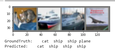
The following code loads numerous samples of the images in the test dataset and then makes some predictions. We use the function torchvision.utils.make_grid() to make a grid of images and display groundtruth and predicted labels. Just follow step by step.
## Define imwshow function
def imshow(img, transpose = True):
    img = img / 2 + 0.5     # unnormalize
    npimg = img.numpy() ## convert image to numpy
    plt.imshow(np.transpose(npimg, (1, 2, 0))) ## The supplied matrix, npimg, ##has to be transposed into numpy with the values of x,y, and z positioned at ##the indexes 1,2,0 respectively.
    plt.show()
## iterate through the dataset. Each iteration returns a batch of images and ##labels
dataiter = iter(testloader)
images, labels = dataiter.next()
# print images
imshow(torchvision.utils.make_grid(images)) ## Display images with ##torchvision.utils.make_grid() function
print('GroundTruth: ', ' '.join('%5s' % classes[labels[j]] for j in range(4))) ## Display labels for ground truth

outputs = net(images) ## outcome prediction for each batch
_, predicted = torch.max(outputs, 1) ## Find the class index that has the ##highest probability and pick that one.

print('Predicted: ', ' '.join('%5s' % classes[predicted[j]] ## Display labels for predicted classes
                              for j in range(4)))
Output:

Let's choose a test image at index ind and run some of our attribution algorithms on it.
ind = 3
input = images[ind].unsqueeze(0) ## adds an additional dimension to the tensor.
input.requires_grad = TrueNote: The most common use for the requires grad_() function is to instruct autograd to start recording operations on a Tensor tensor. If a tensor has the requires_grad=False property (because it was obtained through a DataLoader or required preprocessing or initialization), calling tensor.requires_grad_() will cause autograd to start recording operations on the tensor.
Now, we will set the model to eval mode for interpretation purposes. It is essential to Keep in mind that before starting inference, you need to execute the model.eval() method. Should this step not be taken, the inference outcomes will be inconsistent.
## Set the model in evaluation mode
net.eval()
Output:
Net(
  (conv1): Conv2d(3, 6, kernel_size=(5, 5), stride=(1, 1))
  (pool1): MaxPool2d(kernel_size=2, stride=2, padding=0, dilation=1, ceil_mode=False)
  (pool2): MaxPool2d(kernel_size=2, stride=2, padding=0, dilation=1, ceil_mode=False)
  (conv2): Conv2d(6, 16, kernel_size=(5, 5), stride=(1, 1))
  (fc1): Linear(in_features=400, out_features=120, bias=True)
  (fc2): Linear(in_features=120, out_features=84, bias=True)
  (fc3): Linear(in_features=84, out_features=10, bias=True)
  (relu1): ReLU()
  (relu2): ReLU()
  (relu3): ReLU()
  (relu4): ReLU()
)
Let's define the function for feature attribution.
def attribute_image_f(algorithm, input, **kwargs):
    net.zero_grad()
    tensor_attributions = algorithm.attribute(input,
                                              target=labels[ind],
                                              **kwargs
                                             )

    return tensor_attributions
What are Saliency Maps
Bring this project to life
Saliency maps are visual representations of neural network decision-making processes. They are also helpful in determining a convolutional layer's specific emphasis, giving us a better idea of how decisions are made.
Convolutional neural networks use saliency maps to show us where they're most interested in predicting outcomes.
It is a baseline approach for computing input attribution. It returns the gradients with respect to inputs. The purpose of saliency maps is to emphasize the pixels in the input image that most significantly contributed to the output classification. Now, consider the gradient of the output class score with respect to the pixel values of the input image. The pixels with a significant (positive or negative) gradient are those for which the slightest change is required to impact the class score the most. The object's position in the image may be inferred from these pixels. This is the fundamental concept behind saliency maps. Here, we Compute gradients with respect to class 'ind' and transposes them for visualization purposes.
saliency = Saliency(net)
grads = saliency.attribute(input, target=labels[ind].item())
grads = np.transpose(grads.squeeze().cpu().detach().numpy(), (1, 2, 0))
Integrated Gradients
In their paper titled "Axiomatic Attribution for Deep Networks (ICML 2017)," Mukund Sundararajan, Ankur Taly, and Qiqi Yan investigated the concept of using Integrated Gradients. Through their analysis of the prevalent attribution schemes at the time, the authors focus on two axioms that they believe all feature attribution schemes should adhere to:
- Sensitivity: If each input and baseline differ in one feature yet have different predictions, the differing feature should be assigned a non-zero attribution. It is possible to demonstrate that LRP and DeepLiFT adhere to sensitivity due to the Conservation of Total Relevance. However, the sensitivity Axiom is not guaranteed by gradient-based approaches. When the score function is locally "flat" concerning some input features, saturation occurs at the ReLU or MaxPool stages. A common subject in feature attribution studies is the need to properly transmit relevance or attribution via saturated activations.
- Implementation Invariance: Despite having very different implementations, two networks are considered to be functionally similar if the outputs are identical for all of the inputs. Vanilla gradients theoretically ensure implementation invariance. LRP and DeepLiFT can breach this assumption by using a crude approximation to gradients. The authors provide examples of LRP and DeepLiFT breaking implementation invariance.
The authors suggest employing integrated gradients for feature attribution, which is defined as follows:

The authors demonstrate that the definition mentioned above adheres to both of the desired assumptions:
- Sensitivity: Integrated Gradients, like LRP and DeepLiFT, sum up the difference in feature scores according to the Fundamental Theorem of Calculus. LRP and DeepLiFT are sensitive in the same way.
- Implementation Invariance: Due to its gradient-based definition, it respects the principle of implementation invariance.
We will apply integrated gradients attribution technique to the test image. Integrated Gradients perform the computation necessary to determine the integral of the gradients of the output prediction for the class index ind with respect to the input image pixels.
ig = IntegratedGradients(net)
attrig, delta = attribute_image_f(ig, input, baselines=input * 0, return_convergence_delta=True)
attrig = np.transpose(attrig.squeeze().cpu().detach().numpy(), (1, 2, 0))
print('Approximation delta: ', abs(delta))
Using the test image, the steps required to use integrated gradients and the noise tunnel with the smoothgrad square option are outlined and shown below. Noise Tunnel with smoothgrad square option applies Gaussian noise with a standard deviation of stdevs=0.2 to the input image nt_samples times, computes the attributions for nt_samples images, and then returns the mean of the squared attribution accross nt_samples images.
ig = IntegratedGradients(net)
nt = NoiseTunnel(ig)
attrig_nt = attribute_image_f(nt, input, baselines=input * 0, nt_type='smoothgrad_sq',
                                      nt_samples=100, stdevs=0.2)
attrig_nt = np.transpose(attrig_nt.squeeze(0).cpu().detach().numpy(), (1, 2, 0))
DeepLift
In their work Learning Important Features Through Propagating Activation Differences(ICML 2017), Avanti Shrikumar, Peyton Greenside, and Anshul Kundaje introduced the DeepLiFT approach. These researchers were inspired by Sebastian Bach and his colleagues' studies on the LRP/Taylor decomposition.
Along with an input image, the deep learning algorithm known as DeepLiFT (Deep Learning Important FeaTures) uses a reference image to explain the input pixels.
Even though LRP adhered to the conservation principle, it remained unclear how the net relevance should be distributed over the different pixels. DeepLiFT provides a solution to this issue by enforcing the use of an extra axiom to propagate relevance downward. The following are the two axioms that DeepLiFT adheres to:
- Conservation of Total Relevance: It states that the sum of relevance of all inputs must be equal to the difference in score between the input image score and the baseline image score for every neuron. This axiom is identical to the one that can be found in LRP.
- Chain Rule/Back Propagation: The relevance of each input follows the chain rule like gradients. Using this information, we can use the gradient-like relevance of each input to backpropagate it. This axiom brings DeepLiFT's gradient backpropagation closer to vanilla gradients.
In the code below, we Perform the DeepLift operation on the test image. DeepLIFT explains the difference in output from some ‘reference’ output in terms of the difference of the input from some ‘reference’ input.
dl = DeepLift(net)
attrdl = attribute_image_f(dl, input, baselines=input * 0)
attrdl = np.transpose(attrdl.squeeze(0).cpu().detach().numpy(), (1, 2, 0))
Visualization of Attributions
In the following program, we will see how to visualize the attributions for Saliency Maps, DeepLift, Integrated Gradients, and Integrated Gradients with SmoothGrad. We make use of the function visualize_image_attr, which is responsible for visualizing the attribution of a given image. This is achieved by first normalizing the attribution values of the desired sign (positive, negative, absolute value, or all), and then displaying them in a matplotlib figure using the selected mode.
print('Original Image')
print('Predicted:', classes[predicted[ind]],
      ' Probability:', torch.max(F.softmax(outputs, 1)).item())

original_image = np.transpose((images[ind].cpu().detach().numpy() / 2) + 0.5, (1, 2, 0))

_ = v.visualize_image_attr(None, original_image,
                      method="original_image", title="Original Image")

_ = v.visualize_image_attr(grads, original_image, method="blended_heat_map", sign="absolute_value",
                          show_colorbar=True, title="Overlayed Gradient Magnitudes")

_ = v.visualize_image_attr(attrig, original_image, method="blended_heat_map",sign="all",
                          show_colorbar=True, title="Overlayed Integrated Gradients")

_ = v.visualize_image_attr(attrig_nt, original_image, method="blended_heat_map", sign="absolute_value",
                             outlier_perc=10, show_colorbar=True,
                             title="Overlayed Integrated Gradients \n with SmoothGrad Squared")

_ = v.visualize_image_attr(attrdl, original_image, method="blended_heat_map",sign="all",show_colorbar=True,
title="Overlayed DeepLift")Note: The reader can run the code and visualize the outputs.
Conclusion
In this tutorial, we have shown how to apply model interpretability algorithms from the Captum library on a simple model and test samples from CIFAR dataset. We have built a basic model and use attribution algorithms such as Integrated Gradients, Saliency, DeepLift, and NoiseTunnel to attribute the image's label to the input pixels and visualize it.
References
https://arxiv.org/pdf/1703.01365.pdf
https://debuggercafe.com/saliency-maps-in-convolutional-neural-networks/
https://towardsdatascience.com/explainable-neural-networks-recent-advancements-part-4-73cacc910fef
https://captum.ai/tutorials/CIFAR_TorchVision_Interpret
https://www.oreilly.com/library/view/pytorch-pocket-reference/9781492089995/


