Denoising Autoencoders

In a previous article, I had mentioned how autoencoders may not be the first choice for generative tasks. That being said, they have their own unique strengths. In this article, we will be taking a look at one of those strengths, image denoising.

Setup and imports

#  article dependencies
import torch
import torch.nn as nn
import torch.nn.functional as F
import torchvision
import torchvision.transforms as transforms
import torchvision.datasets as Datasets
from torch.utils.data import Dataset, DataLoader
import numpy as np
import matplotlib.pyplot as plt
import cv2
from tqdm.notebook import tqdm
from tqdm import tqdm as tqdm_regular
import seaborn as sns
from torchvision.utils import make_grid
import random

#  configuring device
if torch.cuda.is_available():
  device = torch.device('cuda:0')
  print('Running on the GPU')
else:
  device = torch.device('cpu')
  print('Running on the CPU')

Autoencoders & Representation Learning

By now, we know that autoencoders learn mappings from input to output for the sole purpose of reconstructing the input data. However, on the surface there really isn't much utility to this.

In the case of convolutional autoencoders, for instance, these autoencoders learn representations in a bid to reconstruct images, you will agree that simply passing an image through a convolutional autoencoder just to get a reconstruction of the same image on the other end isn't too beneficial.

Beyond Image Reconstruction

Keeping with our theme of focusing on image data, consider a case where we have a bunch of corrupted images, images corrupted in the sense that some/all pixels have been modified in some undesirable manner. If one could reproduce this specific form of image corruption such that a dataset of corrupt images is generated from a set of uncorrupted images, a convolutional autoencoder could be trained to learn a mapping from corrupted images to uncorrupted images thereby effectively learning to rid images of this specific form of corruption.

Image corruption in the context mentioned above is called noise, and the process of removing said corruption from images is called image denoising while an autoencoder used to this effect is called a denoising autoencoder.

Implementing a Denoising Autoencoder

In this section, we are going to prepare a dataset for training a denoising autoencoder by adding some noise to images and training a convolutional autoencoder to remove that specific kind of image noise.

Dataset

The CIFAR-10 dataset will be used for training and validation purposes. It is a dataset containing 10 classes of images ranging from frogs to cars, birds etc. It can be loaded in PyTorch as done in the code cell below.

#  loading training data
training_set = Datasets.CIFAR10(root='./', download=True,
                                transform=transforms.ToTensor())

#  loading validation data
validation_set = Datasets.CIFAR10(root='./', download=True, train=False,
                                  transform=transforms.ToTensor())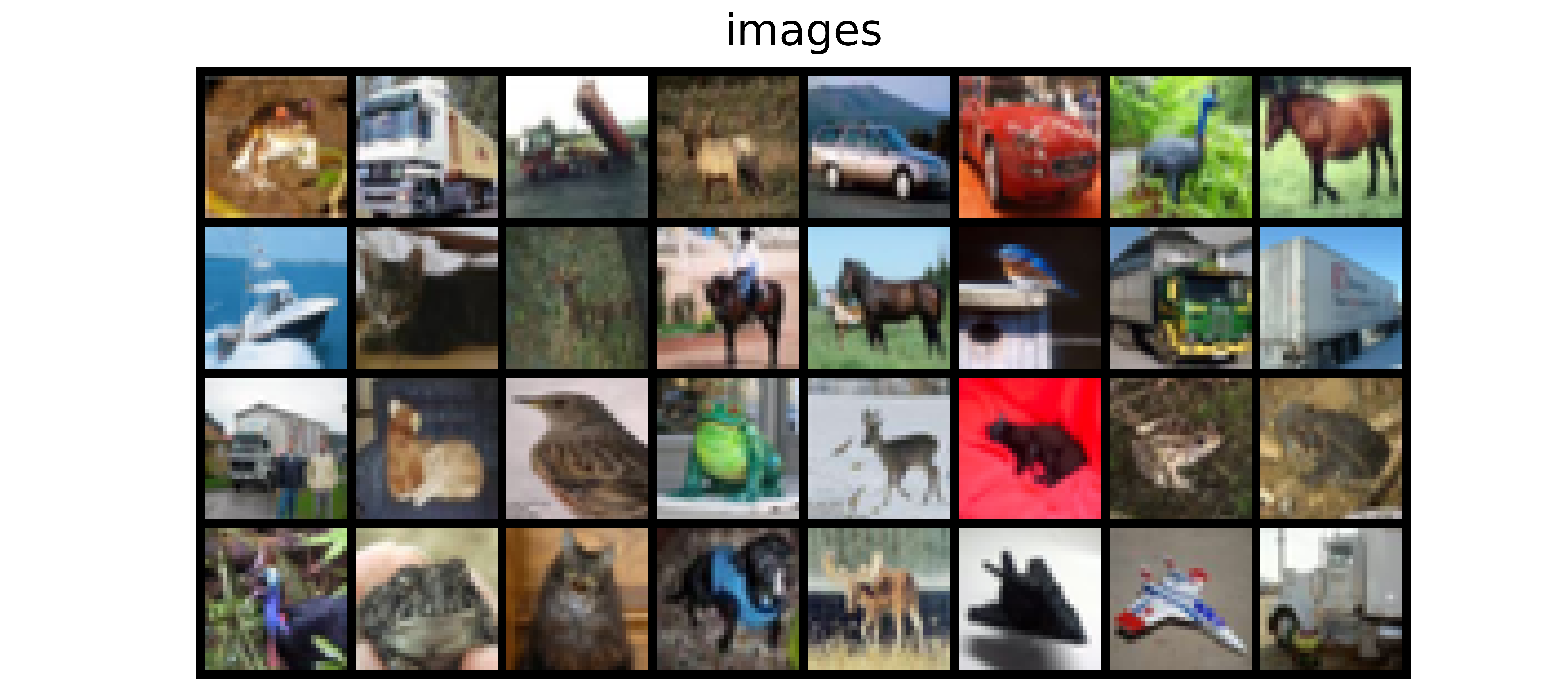

Since we will be learning image to image mapping, we do not need class labels in this case, all that needs to be done is to extract just the training and validation images from their respective objects. Also, for the sake of visualization we will extract one image from each class in the validation set so we can see how well the autoencoder does at denoising images of that class after each epoch when training, we will call this the test set.

def extract_each_class(dataset):
  """
  This function searches for and returns
  one image per class
  """
  images = []
  ITERATE = True
  i = 0
  j = 0

  while ITERATE:
    for label in tqdm_regular(dataset.targets):
      if label==j:
        images.append(dataset.data[i])
        print(f'class {j} found')
        i+=1
        j+=1
        if j==10:
          ITERATE = False
      else:
        i+=1

  return images
  
  
#  extracting training images
training_images = [x for x in training_set.data]

#  extracting validation images
validation_images = [x for x in validation_set.data]

#  extracting one image from each class in the validation set
test_images = extract_each_class(validation_set)

Image to Grayscale

While there are different types of image noises, in this article we will focus on 'salt and pepper noise', a kind of noise which prevalently occurs in grayscale images. As we know, CIFAR-10 images are colored, in order to easily convert them to grayscale we can simply take the mean of individual pixels across channels so we go from a 3 channel image (color) to a single channel image (grayscale).

#  converting images to grayscale by taking mean across axis-2 (depth)
training_gray = [x.mean(axis=2) for x in training_images]
validation_gray = [x.mean(axis=2) for x in validation_images]
test_gray = [x.mean(axis=2) for x in test_images]

In a bid to clean up pixel values a little bit, let's normalize pixels by constraining them to values between 0 and 1 which is typical for most gray scale images.

def min_max_normalize_gray(dataset: list):
  """
  This function normalizes data by constraining
  data points between the range of 0 & 1  
  """
  #  create a list to hold normalized data  
  normalized = []

  for image in tqdm_regular(dataset):
    #  creating temporary store
    temp = []
    #  flatenning
    pixels = image.flatten()
    #  derive minimum and maximum values
    minimum = pixels.min()
    maximum = pixels.max()
    #  convert to list for iteration
    pixels = list(pixels)

    for pixel in pixels:
      #  normalizing pixels
      normalize = (pixel-minimum)/(maximum-minimum)
      #  appending each pixel to temporary store
      temp.append(round(normalize, 2))

    temp = np.array(temp)
    temp = temp.reshape((32, 32))
    #  appending normalized image to list
    normalized.append(temp)
  
  return normalized
  
  
#  normalizing pixels
training_gray = min_max_normalize_gray(training_gray)
validation_gray = min_max_normalize_gray(validation_gray)
test_gray = min_max_normalize_gray(test_gray)

Creating Noisy Copies

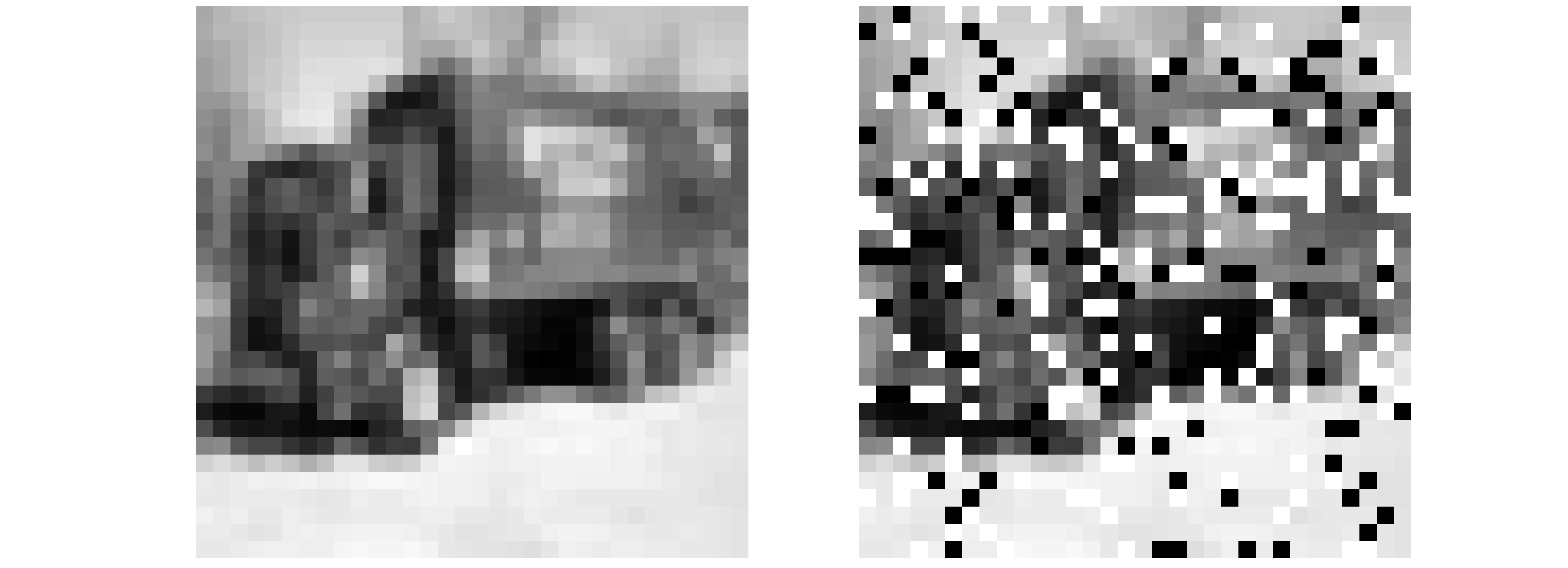
Salt and pepper noise can be thought of as specks of white (salt) and black (pepper) pixels 'sprinkled' across the surface of an image. Conceptually this simply means some pixels have been casted to o (black) and 1 (white) at random. Armed with this knowledge, we can reproduce salt and pepper noise using the code cell below.

def random_noise(dataset: list, noise_intensity=0.2):
  """
  This function replicates the salt and pepper noise process
  """
  noised = []
  noise_threshold = 1 - noise_intensity

  for image in tqdm_regular(dataset):
    #  flatenning image
    image = image.reshape(1024)

    #  creating vector of zeros
    noise_vector = np.zeros(1024)

    #  noise probability
    for idx in range(1024):
      regulator = round(random.random(), 1)
      if regulator > noise_threshold:
        noise_vector[idx] = 1
      elif regulator == noise_threshold:
        noise_vector[idx] = 0
      else:
        noise_vector[idx] = image[idx]
    
    #  reshaping noise vectors
    noise_vector = noise_vector.reshape((32, 32))

    noised.append(noise_vector)
  return noised
  
  
#  adding noise to images
training_noised = random_noise(training_gray)
validation_noised = random_noise(validation_gray)
test_noised = random_noise(test_gray)

Visualizing the noisy images from the above defined process shows the presence of white and black specks emulating salt and pepper noise. As images in the CIFAR-10 dataset are of size 32 x 32 pixels, pardon the heavy pixelation.

The training, validation and test sets can now be put together by zipping the corrupted and uncorrupted images to form an image-target pair as done in the code cell below.

#  creating image-target pair
training_set = list(zip(training_noised, training_gray))
validation_set = list(zip(validation_noised, validation_gray))
test_set = list(zip(test_noised, test_gray))

PyTorch Dataset

In order to use our dataset in PyTorch, we need to instantiate it as a member of a PyTorch dataset class as done below. Note that pixels in the images are again normalized around a mean of 0.5 and a standard deviation of 0.5 in a bid to put all pixels within an manageable approximate distribution.

#  defining dataset class
class CustomCIFAR10(Dataset):
  def __init__(self, data, transforms=None):
    self.data = data
    self.transforms = transforms

  def __len__(self):
    return len(self.data)

  def __getitem__(self, idx):
    image = self.data[idx][0]
    target = self.data[idx][1]

    if self.transforms!=None:
      image = self.transforms(image)
      target = self.transforms(target)
    return (image, target)
    
    
#  creating pytorch datasets
training_data = CustomCIFAR10(training_set, transforms=transforms.Compose([transforms.ToTensor(),
                                                                          transforms.Normalize(0.5, 0.5)]))
validation_data = CustomCIFAR10(validation_set, transforms=transforms.Compose([transforms.ToTensor(),
                                                                              transforms.Normalize(0.5, 0.5)]))
test_data = CustomCIFAR10(test_set, transforms=transforms.Compose([transforms.ToTensor(),
                                                                  transforms.Normalize(0.5, 0.5)]))

Piecing Together a Convolutional Autoencoder

A convolutional autoencoder now needs to be defined. For this article, we will be implementing the custom built autoencoder architecture illustrated in the image below.

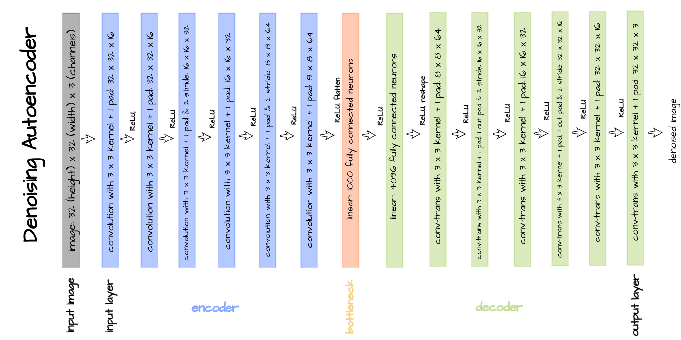
This autoencoder is made up of an encoder and a decoder with 6 convolution layers each. A bottleneck/latent space of size 1000 is also specified. The architecture is implemented in PyTorch as seen in the code cell below.

#  defining encoder
class Encoder(nn.Module):
  def __init__(self, in_channels=3, out_channels=16, latent_dim=1000, act_fn=nn.ReLU()):
    super().__init__()
    self.in_channels = in_channels

    self.net = nn.Sequential(
        nn.Conv2d(in_channels, out_channels, 3, padding=1), # (32, 32)
        act_fn,
        nn.Conv2d(out_channels, out_channels, 3, padding=1), 
        act_fn,
        nn.Conv2d(out_channels, 2*out_channels, 3, padding=1, stride=2), # (16, 16)
        act_fn,
        nn.Conv2d(2*out_channels, 2*out_channels, 3, padding=1),
        act_fn,
        nn.Conv2d(2*out_channels, 4*out_channels, 3, padding=1, stride=2), # (8, 8)
        act_fn,
        nn.Conv2d(4*out_channels, 4*out_channels, 3, padding=1),
        act_fn,
        nn.Flatten(),
        nn.Linear(4*out_channels*8*8, latent_dim),
        act_fn
    )

  def forward(self, x):
    x = x.view(-1, self.in_channels, 32, 32)
    output = self.net(x)
    return output


#  defining decoder
class Decoder(nn.Module):
  def __init__(self, in_channels=3, out_channels=16, latent_dim=1000, act_fn=nn.ReLU()):
    super().__init__()

    self.out_channels = out_channels

    self.linear = nn.Sequential(
        nn.Linear(latent_dim, 4*out_channels*8*8),
        act_fn
    )

    self.conv = nn.Sequential(
        nn.ConvTranspose2d(4*out_channels, 4*out_channels, 3, padding=1), # (8, 8)
        act_fn,
        nn.ConvTranspose2d(4*out_channels, 2*out_channels, 3, padding=1, 
                           stride=2, output_padding=1), # (16, 16)
        act_fn,
        nn.ConvTranspose2d(2*out_channels, 2*out_channels, 3, padding=1),
        act_fn,
        nn.ConvTranspose2d(2*out_channels, out_channels, 3, padding=1, 
                           stride=2, output_padding=1), # (32, 32)
        act_fn,
        nn.ConvTranspose2d(out_channels, out_channels, 3, padding=1),
        act_fn,
        nn.ConvTranspose2d(out_channels, in_channels, 3, padding=1)
    )

  def forward(self, x):
    output = self.linear(x)
    output = output.view(-1, 4*self.out_channels, 8, 8)
    output = self.conv(output)
    return output


#  defining autoencoder
class Autoencoder(nn.Module):
  def __init__(self, encoder, decoder):
    super().__init__()
    self.encoder = encoder
    self.encoder.to(device)

    self.decoder = decoder
    self.decoder.to(device)

  def forward(self, x):
    encoded = self.encoder(x)
    decoded = self.decoder(encoded)
    return decoded

Convolutional Autoencoder Class

A typical autoencoder performs 3 main functions, it learns a vector representation via it's encoder, this representation is compressed in it's bottleneck before the image is reconstructed by it's decoder. So as to be able to use these individual components of an autoencoder separately if need be, we will define a class which helps to facilitate this by defining two of those functions as methods. For portability, a training method will also be built into this class.  

#  defining class
class ConvolutionalAutoencoder():
  def __init__(self, autoencoder):
    self.network = autoencoder
    self.optimizer = torch.optim.Adam(self.network.parameters(), lr=1e-3)

  def train(self, loss_function, epochs, batch_size, 
            training_set, validation_set, test_set,
            image_channels=3):
    
    #  creating log
    log_dict = {
        'training_loss_per_batch': [],
        'validation_loss_per_batch': [],
        'visualizations': []
    } 

    #  defining weight initialization function
    def init_weights(module):
      if isinstance(module, nn.Conv2d):
        torch.nn.init.xavier_uniform_(module.weight)
        module.bias.data.fill_(0.01)
      elif isinstance(module, nn.Linear):
        torch.nn.init.xavier_uniform_(module.weight)
        module.bias.data.fill_(0.01)

    #  initializing network weights
    self.network.apply(init_weights)

    #  creating dataloaders
    train_loader = DataLoader(training_set, batch_size)
    val_loader = DataLoader(validation_set, batch_size)
    test_loader = DataLoader(test_set, 10)

    #  setting convnet to training mode
    self.network.train()
    self.network.to(device)

    for epoch in range(epochs):
      print(f'Epoch {epoch+1}/{epochs}')
      train_losses = []

      #------------
      #  TRAINING
      #------------
      print('training...')
      for images, targets in tqdm(train_loader):
        #  zeroing gradients
        self.optimizer.zero_grad()
        #  sending images and targets to device
        images = images.to(device).type(torch.cuda.FloatTensor)
        targets = targets.to(device).type(torch.cuda.FloatTensor)
        #  reconstructing images
        output = self.network(images)
        #  computing loss
        loss = loss_function(output, targets)
        loss = loss#.type(torch.cuda.FloatTensor)
        #  calculating gradients
        loss.backward()
        #  optimizing weights
        self.optimizer.step()

        #--------------
        # LOGGING
        #--------------
        log_dict['training_loss_per_batch'].append(loss.item())

      #--------------
      # VALIDATION
      #--------------
      print('validating...')
      for val_images, val_targets in tqdm(val_loader):
        with torch.no_grad():
          #  sending validation images and targets to device
          val_images = val_images.to(device).type(torch.cuda.FloatTensor)
          val_targets = val_targets.to(device).type(torch.cuda.FloatTensor)
          #  reconstructing images
          output = self.network(val_images)
          #  computing validation loss
          val_loss = loss_function(output, val_targets)

        #--------------
        # LOGGING
        #--------------
        log_dict['validation_loss_per_batch'].append(val_loss.item())


      #--------------
      # VISUALISATION
      #--------------
      print(f'training_loss: {round(loss.item(), 4)} validation_loss: {round(val_loss.item(), 4)}')

      for test_images, test_targets in test_loader:
        #  sending test images to device
        test_images = test_images.to(device).type(torch.cuda.FloatTensor)
        with torch.no_grad():
          #  reconstructing test images
          reconstructed_imgs = self.network(test_images)
        #  sending reconstructed and images to cpu to allow for visualization
        reconstructed_imgs = reconstructed_imgs.cpu()
        test_images = test_images.cpu()

        #  visualisation
        imgs = torch.stack([test_images.view(-1, image_channels, 32, 32), reconstructed_imgs], 
                          dim=1).flatten(0,1)
        grid = make_grid(imgs, nrow=10, normalize=True, padding=1)
        grid = grid.permute(1, 2, 0)
        plt.figure(dpi=170)
        plt.title('Original/Reconstructed')
        plt.imshow(grid)
        log_dict['visualizations'].append(grid)
        plt.axis('off')
        plt.show()
      
    return log_dict

  def autoencode(self, x):
    return self.network(x)

  def encode(self, x):
    encoder = self.network.encoder
    return encoder(x)
  
  def decode(self, x):
    decoder = self.network.decoder
    return decoder(x)

Training a Denoising Autoencoder

Now a denoising autoencoder is ready to be trained. Training is done by instantiating the autoencoder class as a member of the convolutional autoencoder class and calling the train method. Mean squared error is used as the loss function of choice as the model is trained for 15 epochs using a batch size of 64.

#  training model
model = ConvolutionalAutoencoder(Autoencoder(Encoder(in_channels=1),
                                               Decoder(in_channels=1)))

log_dict = model.train(nn.MSELoss(), epochs=15, batch_size=64, 
                       training_set=training_data, validation_set=validation_data,
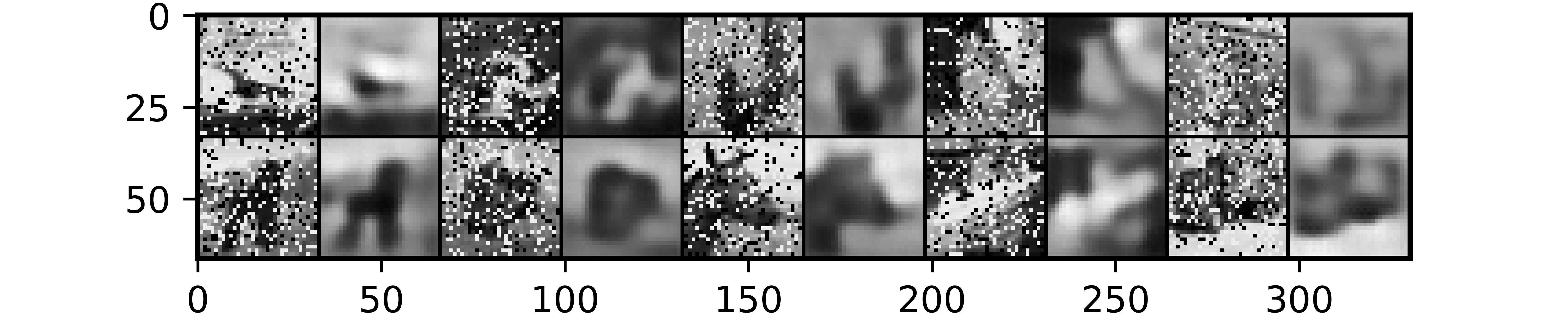
                       test_set=test_data, image_channels=1)

After the first epoch, it is evident that the autoencoder is already doing a decent job at removing the noise/corruption from images as seen in the visualization returned after each epoch. It's reconstructions are however very low detail (blurry).

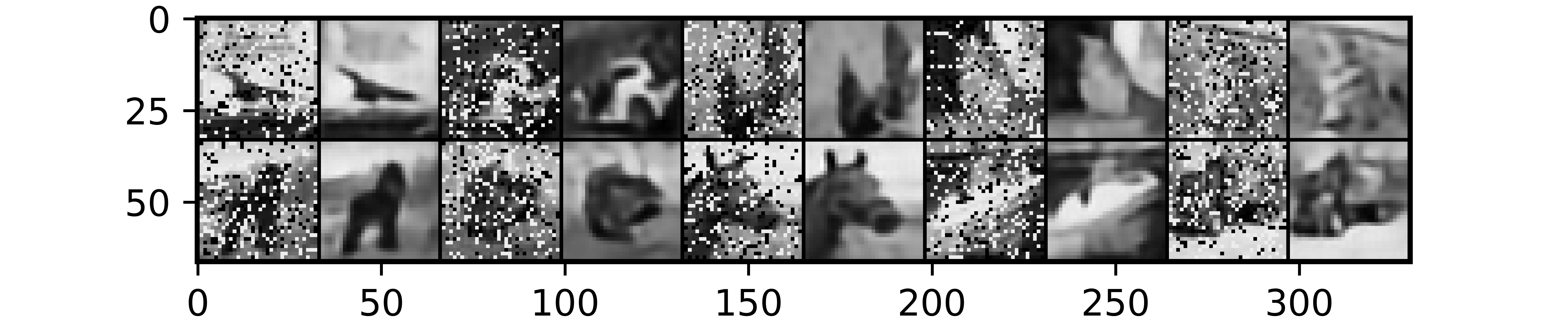
Training for more epochs ensures that a more refined reconstruction is produced and by the 15th epoch a clear upgrade is seen in the quality of denoised images as compared to epoch 1. It is imperative to remember that images denoised in the visualizations are test images which the autoencoder was not trained on, a testament to it's generalization.

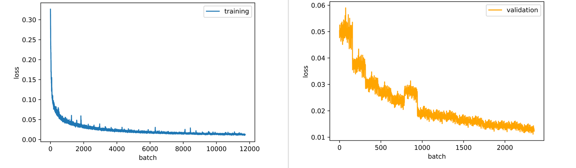
Taking a look at the training and validation loss plots, it is evident that both losses are down-trending therefore implying that the autoencoder could still benefit from some additional epochs of training.

Final Remarks

In this article we took a look at one of the uses of autoencoders which is image denoising. We were able to see how an autoencoder's representation learning allows it to learn mappings efficient enough to fix incorrect pixels/datapoints.

This could be extended as far as tabular data applications where there are some cases where autoencoders have been beneficial in helping to fill missing values in data instances. It should however be noted that denoising autoencoders only work on the specific kind of noise they have been trained on.