Spam or Ham?

Most of the data we generate is unstructured. This includes sources like text, audio, video, and images which an algorithm might not immediately comprehend. Yet, imagine if a human had to individually sort each and every email into your inbox or spam folder! Luckily, one of the most exciting areas of data science generally and machine learning specifically is the task of wrangling such sources of data and finding ways to perform meaningful analysis on this data.
In this article, we'll construct a spam filter which we can use to classify text messages as ham or spam -- that is, legitimate versus junk mail messages. This example will introduce text as a source of data, as well as help to illustrate some common machine learning concepts. Although this tutorial is designed for beginners, more seasoned users who are less familiar with but interested in the R statistical language might find this implementation helpful. Please feel free to code along!
Some basics of textual data in R
To construct a spam filter, we first need to transform our plain text messages into a format which our model can comprehend. Specifically, we need to represent our text messages as word counts or frequencies. Once represented in this format, then a variety of statistical models and procedures are available to make sense of this data. This is known as natural language processing.
We can do this by first loading text files into a statistical software package. This tutorial will use the powerful and widely-used statistical language R and implement this through R Studio. For more information on installing and setting up R on your machine, check out this link. The software and packages you'll need are all open source.
Let's load two packages: quanteda and RColorBrewer. The former is a popular package for the statistical analysis of textual data, and the latter provides a suite of coloring options for the graphics we'll produce. The library() command instructs R to load these packages if they have already been installed. If you're new to R (or these packages), then replace this command with install.packages("") to install these packages before accessing them from your library.
library(quanteda)
library(RColorBrewer)
With our packages loaded, let's import a publicly available SMS spam/ham dataset from here, which was introduced in Almeida et al.
We know from the README file that this dataset is represented as a single plain text file which lists the content of SMS messages with an associated label of ham or spam. There are 5,574 SMS messages, of which 13.4% are spam and 86.6% are legitimate messages. Our challenge is to construct a supervised machine learning classifier which can separate the two types all on its own.
First download the data from the above URL, and then set your R working directory to the folder in which you downloaded the file. This tells R where to look for the data on your computer. Finally, read the data into R using the read.table command and specify the file name in quotation marks. The other arguments in the parentheses tell R how to read the plain text file. We'll name this collection of SMS messages "raw.data" by using <-.
setwd("~/Your Folder Path")
raw.data <- read.table("SMSSpamCollection", header=FALSE, sep="\t", quote="", stringsAsFactors=FALSE)
If you encounter any error messages while trying to import your data, check out StackExchange or StackOverflow for helpful advice. Actually, data import can be one of the more tedious tasks!
Let's add headers to the two columns of information. We'll call the first column "Label" and the second column "Text". This will allow us to easily remember and call up these variables later in the analysis. Finally, we can check out the number of ham and spam messages to double check that our data imported properly.
names(raw.data) <- c("Label", "Text")
table(raw.data$Label)
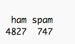
It looks like we're dealing with 4,827 ham messages and 747 spam messages. This checks out with the description of the data in the dataset's README file, so we should be good to go.
The last thing we'll do at the data import phase is to randomize our data using the sample() command. Just in case the data are not stored in a random distribution, this will help to ensure that we are dealing with a random draw from our data. The set.seed() command is simply there to ensure more consistent replication, so that your results should mirror the results found in this tutorial.
set.seed(1912)
raw.data <- raw.data[sample(nrow(raw.data)),]
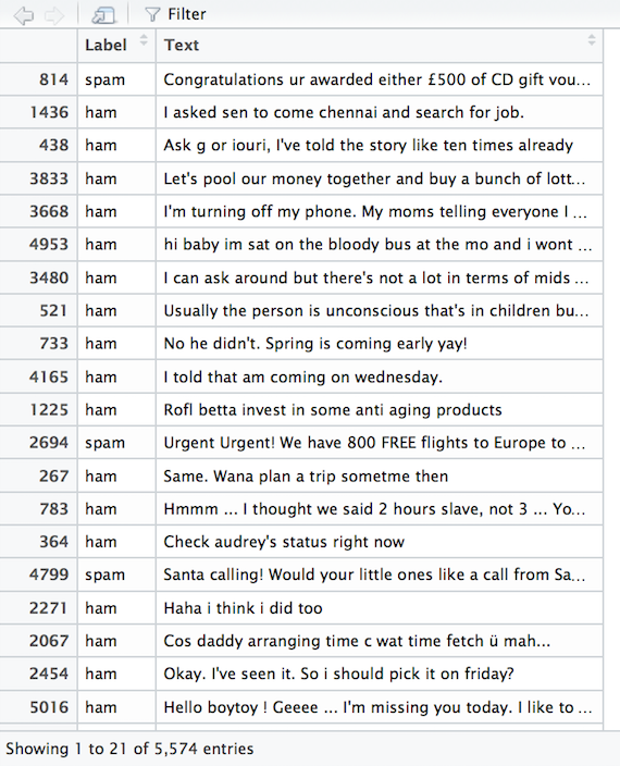
You can check out what the data looks like by using the View() command. You'll notice that we've turned a plain text file into a nicely stored data frame complete with labeled headers and randomized observations.
Before we jump into building the classification model, let's get a feel for our data using an intuitive visualization: the word cloud. We can then visually inspect the image to see whether there seems to be a difference in the language between the ham and spam messages.
In natural language processing, we like to deal with corpus objects. A corpus can be thought of as a master copy of our dataset from which we can pull subsets or observations as needed. We'll use quanteda's corpus() command to construct a corpus from the Text field of our raw data, which we can name sms.corpus. Then, attach the Label field as a document variable to the corpus using the docvars() command. We attach Label as a variable directly to our corpus so that we can associate SMS messages with their respective ham/spam label later in the analysis.
sms.corpus <- corpus(raw.data$Text)
docvars(sms.corpus) <- raw.data$Label
With our master corpus constructed, we can now subset this into spam and ham messages to construct word clouds and have a look at the differences in language they use. The larger the word displays, the more frequent that word appears in our data.
First, subset the corpus into spam. Remember, we need to convert these words into something that the computer can count. So, construct a document term frequency matrix (DFM) using the dfm() command and remove some clutter, such as punctuation, numbers, and commonly occurring words which might possess little meaningful information. This is called a bag-of-words approach.
spam.plot <- corpus_subset(sms.corpus, docvar1 == "spam")
spam.plot <- dfm(spam.plot, tolower = TRUE, removePunct = TRUE, removeTwitter = TRUE, removeNumbers = TRUE, remove=stopwords("SMART"))
With our DFM constructed, let's plot the spam word cloud. We'll use the brewer.pal command from the RColorBrewer package to color our word plot according to word frequency. We can add a title to the plot, too.
spam.col <- brewer.pal(10, "BrBG")
spam.cloud <- textplot_wordcloud(spam.plot, min.freq = 16, color = spam.col)
title("Spam Wordcloud", col.main = "grey14")
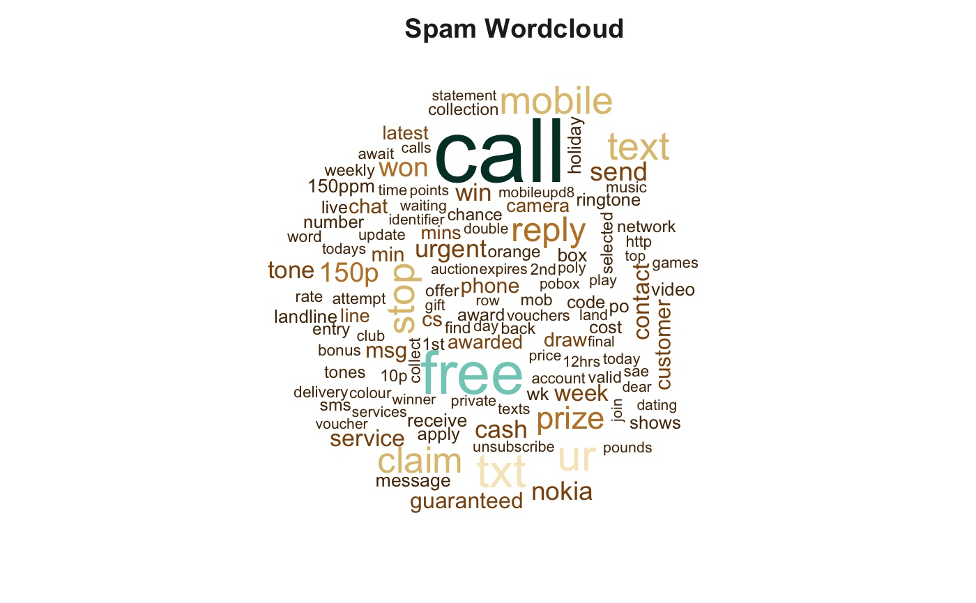
Notice words like "free", "urgent", and "customer". These are words that might intuitively come to mind when thinking about spam messages, so we might be on to something. We can now repeat this coding process for the ham messages and compare the two clouds.
ham.plot <- corpus_subset(sms.corpus, docvar1 == "ham")
ham.plot <- dfm(ham.plot, tolower = TRUE, removePunct = TRUE, removeTwitter = TRUE, removeNumbers = TRUE, remove=c("gt", "lt", stopwords("SMART")))
ham.col <- brewer.pal(10, "BrBG")
textplot_wordcloud(ham.plot, min.freq = 50, colors = ham.col, fixed.asp = TRUE)
title("Ham Wordcloud", col.main = "grey14")
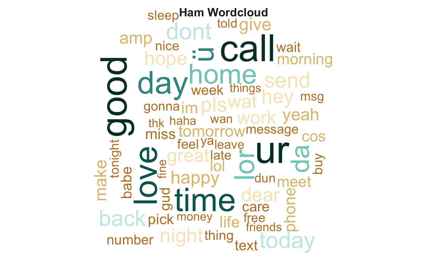
Notice words like "home", "time", and "love". This seems to be much more personal language than the words popping up in the spam set. Our intuition -- that the words used in these messages should be different -- seems to check out. Let's now proceed to constructing a machine learning model which can be used to automatically classify messages into ham or spam categories.
DIY: Constructing a spam filter
Imagine that you're reading through reviews for a new movie. You'll notice that some of the five star reviews include words like "excellent" or "superb". Perhaps some of the one star reviews include words like "horrible" or "awful". In fact, you'll get so good at reading movie reviews that you might be able to accurately predict the star rating associated with a given review simply based on the types of words that reviewer uses.
This is the intuition behind our task. In machine learning, this is called a "supervised" learning problem. More specifically, it is also called a "classification" task. It is supervised, because you offer the model supervision: you train the model on data labeled as spam or ham so that it can learn what a spam or ham message looks like. It is a classification problem, because the model then tries to classify new text messages as spam or ham based on the content of those new text messages.
We can use a simple naive Bayes classifier for this task. For more information on Bayesian classifiers, see this StackOverflow post. In short, Bayesian classifiers are simple probabilistic classifiers based on Bayes' theorem with strong feature independence assumptions.
We've already imported our text messages as a corpus -- the master copy of the data -- so the next step is to represent the text messages as word counts in the form of a DFM. Typically, we would want to discard punctuation, numbers, and commons words since these often offer little predictive capability. In the case of classifying SMS messages, though, researchers have found that including such information boosts performance. So, we'll only minimally pre-process this data and weight the word counts.
sms.dfm <- dfm(sms.corpus, tolower = TRUE)
sms.dfm <- dfm_trim(sms.dfm, min_count = 5, min_docfreq = 3)
sms.dfm <- dfm_weight(sms.dfm, type = "tfidf")
Now, we need to split our data into training and test samples. The training sample trains our model, i.e. helps it learn what ham and spam look like. The test sample can then be used to test the model to see how well it performs. Let's use 85% of our data to train our model, and see how well it can predict the spam or ham labels of the remaining 15% of the data.
In R, we can subset data by calling up the data name and alter it using square brackets. The first 85% of our data approximately corresponds to the 4,738th observation. The remaining 15% will then be number 4,739 to the final row (i.e. nrow() of the dataset). We'll do this to both the raw.data and our DFM so that we have everything required for our model.
sms.raw.train <- raw.data[1:4738,]
sms.raw.test <- raw.data[4739:nrow(raw.data),]

sms.dfm.train <- sms.dfm[1:4738,]
sms.dfm.test <- sms.dfm[4739:nrow(raw.data),]
With our data split into training and test data sets, we'll train our naive Bayes model, and tell the model to pay attention to the content of the text message and the ham or spam label of the message. Then, we'll use that trained model to predict whether the new test observations are ham or spam all on its own. Finally, we'll make a contingency table to see how accurately it performs.
The quanteda package allows us to directly access a naive Bayes classification model using the textmodel_NB command. We plug in our training DFM, which we named sms.dfm.train and the vector of labels associated with the training documents using sms.raw.train$Label. We'll call this our sms.classifier.
sms.classifier <- textmodel_NB(sms.dfm.train, sms.raw.train$Label)
This produces a fitted model, i.e. a classifier which as been trained. Let's now use this model to predict the spam/ham labels of our test data. This means that we only feed this model the textual information without labels. We can do this by passing our fitted model -- sms.classifier -- through the predict() command, specifying our sms.dfm.test data as the new data on which to make predictions. Finally, the table command allows us to view the results of our model's predictions.
sms.predictions <- predict(sms.classifier, newdata = sms.dfm.test)
table(sms.predictions$nb.predicted, sms.raw.test$Label)
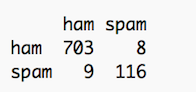
This table should be read from left to right: the model classified 703 ham messages correctly as ham, and 8 ham messages incorrectly as spam. The model incorrectly classified 9 spam messages as ham, but 116 spam messages correctly as spam.
By dividing the correct number of classifications by the total number of classifications attempted, we find that our model correctly classifies 98.9% of ham messages and 92.8% of spam messages. So, for every 100 messages you receive, one legitimate message might accidentally end up in your spam folder. If you receive 100 spam messages, seven of those might sneak through the spam filter and end up in your inbox. This is quite impressive for a simple classifier! For more information on evaluating the model, check out this StackExchange post.
Concluding notes
In this tutorial, we briefly discussed the treatment of text as data and walked through the process of importing and visualizing this data in R. We also outlined the logic of supervised classification problems in machine learning and illustrated these concepts through the construction of a simple spam filter.
This example is just one of many applications for the analysis of textual data. If you're interested in this topic, read up on the quanteda package for R, as well as the tm package for text mining and the RTextTools package for machine learning classification of text. Readers interested in implementing statistical procedures more generally might find the popular e1071 package to be helpful. More info on the dataset and related research can be found from this paper and this paper.
Hopefully, seeing these machine learning concepts in action helps to make their intuition and application more concrete. Perhaps it also illustrates the potential of these models -- we built a relatively accurate model capable of sorting hundreds of text messages on its own and in less than one second. Thanks for reading and happy coding!
To get started with your own R setup, sign up here.