Access to humongous amounts of data and the availability of enormous computational power have led us to explore various techniques to draw out useful patterns and lead better lives. Churning the data rightly has become a necessity. Industrial automation, disease detection in healthcare, robotics, resource management, and personalized recommendations have paved their way into our lives. They have revolutionized our clichéd ways of perceiving and executing tasks. By the same token, Reinforcement Learning, a subfield of Machine Learning, has carved a niche in the current technical era by promoting automated decision-making.
Here’s a list of topics that we will be going through to understand Reinforcement Learning in detail:
- It All Started with Machine Learning
- The Essence of Reinforcement Learning
- RL in Robotics
- Other Applications of RL
- Markov Decision Process (MDP)
- Optimal Policy Search
- Monte-Carlo Learning
- Dynamic Programming
- Temporal-Difference Learning
- Q-Learning
- Exploration-Exploitation Trade-Off
- Epsilon-Greedy Exploration Policy
- Deep Q-Networks
- Conclusion
Bring this project to life
It All Started with Machine Learning
Machine Learning, as the name suggests, gives machines the capability to learn without explicit programming. Given a set of observational data points, a machine formulates a decision comparable to how a human formulates one.
Supervised Learning in Machine Learning is the availability of labels for the data points. For example, if we consider the Iris dataset (comprised of plant features and their corresponding plant names), the supervised learning algorithm has to learn the mapping between features and labels, and output the label given a sample.
Unsupervised Learning in Machine Learning is the non-use of labels. It’s the responsibility of the algorithm to derive patterns from the data by analyzing the probability distribution.
Reinforcement Learning (RL) in Machine Learning is the partial availability of labels. The learning process is similar to the nurturement that a child goes through. A parent nurtures the child, approving or disapproving of the actions that a child takes. The child learns and acts accordingly. Eventually, the child learns to maximize the success rate by inclining towards actions for which there's positive feedback. This is how Reinforcement Learning proceeds. It is a technique comparable to human learning, which gained momentum in the recent decade due to its proximity to human actions and perceptions.
The Essence of Reinforcement Learning
Reinforcement Learning helps in formulating the best decisions, closing in on the success measure. Every action isn’t supervised; instead the machine has to learn by itself to near the success rate.
There are four primary components in Reinforcement Learning:
- Agent: The entity which has to formulate the decisions.
- Action: The events performed by an entity.
- Environment: The scenario in which an agent performs an action. It’s bound by a set of rules where the environment responds for every action.
- Reward: Feedback mechanism that notifies the agent about the success rate.

RL in Robotics
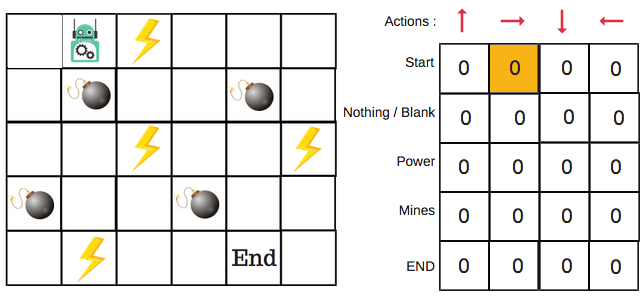
A phenomenal RL application is in the Robotics field. A robot has to have the intelligence to perform unknown tasks when no success measure is given. It has to explore all the possibilities and reach its destined goal. If we consider the typical Reinforcement Learning nomenclature, a robot here is an agent. The action is its movement. The environment is, say, a maze. The reward is the points that it receives on making a successful move. All the four components taken together explain a Reinforcement Learning scenario.
Other Applications of RL
Besides Robotics, RL has proved to be a promising technique in achieving state-of-the-art solutions in various other fields:
- Autonomous Driving - Parking a car, moving the car in the right directions, trajectory optimization, motion planning, scenario-based learning, etc.
- Traffic Light Control - Controlling the traffic lights according to the number of vehicles on road.
- Healthcare - Find optimal treatment schedules and design better prosthetics.
- Finance - Trading and price optimization.
- Power Systems - Reduce energy consumption by utilizing effective energy consumption strategies.
- Gaming - Tremendous outcomes have come from using Reinforcement Learning in the gaming industry. AlphaGo Zero and Dota 2 have been played by agents trained on reinforcement learning algorithms, which performed quite well.
Markov Decision Processes (MDP)
A Markov Decision Process presents an environment to the reinforcement learning agent. To understand Markov Decision Processes, let’s first comprehend their prerequisites.
A Markov Property is a memoryless property that depends on the current state, but not on the previous states (it assumes that the present is a holistic representation of all past events). In other words., the future doesn’t depend upon the past, given the present. A process possessing such a property is called a Markov Process. A process here is a sequence of states $S1, S2, S3,...$ possessing a Markov property. It is defined using two parameters: the state $S$ and the transition function $P$ (i.e. the function to transition from one state to the other).
A Markov Reward Process defines the reward accumulated for a Markov Process. It is defined by state $S$, transition function $P$, reward $R$, and a discount rate $D$. $D$ explains the rewards in the future, given a reward in the present. If $D$ is 0, the agent cares only about the next reward. If $D$ is 1, the agent cares about all future rewards. The discount factor $D$ is necessary to converge the outcome, which could otherwise lead to infinitely mundane results.
The overall reward accumulated from a given time $t$ is given by a simple mathematical equation:
$$R_t = R_{t+1} + DR_{t+2} + D^2R_{t+3} + …$$
If $D$ = 0, $R_t = R_{t + 1}$ and the agent only cares about the next reward.
If $D$ = 1, $R_t = R_{t+1} + R_{t+2} + …$ and the agent cares about all the future awards.
A Markov Decision Process (MDP) is a Markov Reward Process applied to decisions. It’s represented by a state $S$, transition function $P$, reward $R$, discount rate $D$, and a set of actions $a$. A MDP could be assumed as an interface between an agent and the environment. An agent performs a specific set of actions in an environment, which then responds with a reward and a new state. The next state and reward depend only on the previous state and action.
Optimal Policy Search
Now that the environment is defined using MDP, our focus has to be on maximizing the reward. To achieve this, the agent has to determine the best action at every state that it will be in, or in general, determine the the best policy or strategy.
The Bellman Equation helps in estimating the value of each state by computing the future rewards that the state can generate.
$$V^{}(S) = max_a \sum_{S^{'}}P(S, a, S^{'})[R(S, a, S^{'}) + D V(S{'})]$$
Where:
- $P(S, a, S^{’})$ is the transition probability from state $S$ to $S^{’}$ when the action is $a$
- $R(S, a, S^{’})$ is the reward obtained transitioning from state $S$ to $S^{’}$ when the action is $a$
- D is the discount factor
- $V(S^{’})$ is the value of state $S{’}$
The above equation can be obtained from Markov’s equation as follows.
$R_t = R_{t+1} + DR_{t+2} + D^2R_{t+3} + …$
$R_t = R_{t+1} + D(R_{t+2} + DR_{t+3} + …)$
$R_t = R_{t+1} + DR_{t+1}$
The expected value (EV) would then be:
$$V^{}(S) = max_a \sum_{S^{'}}P(S, a, S^{'})[R(S, a, S^{'}) + D V(S{'})]$$
The Bellman Equation computes the optimal state, which along with a paired action shall further enhance the optimal policy search. This can be achieved using the Q-Value.
The Q-value defines the action that has to be chosen by the agent in a particular state. The Q-value can be computed using the following equation:
$$Q_{k+1}(S, a) = \sum_{S^{'}} P(S, a, S^{'})[R(S, a, S^{'}) + D.max_{a^{'}} Q_{k}(S^{'},a^{'})] \forall (S, a) $$
Where $max_{a^{'}} Q_{k}(S^{'}, a^{'})$ defines the action $a^{'}$ taken at state $S^{'}$.
In short, the training of agents happens iteratively by computing the results using the Bellman Equation (optimal state) and the Q-value (optimal action).
Monte-Carlo Learning
Our assumption in the optimal policy search is that the probability is included, though the value is not known to us. Hence to find the probability, the agent has to interact with the environment and find all the possible probabilities of transitioning from one state to the other.
Monte-Carlo is a technique that randomly samples the inputs to determine the output which is closer to the reward under consideration. It generates a trajectory that updates the action-value pair according to the reward observed. Eventually, the policy/trajectory converges to the optimal goal.
Every trial (random sampling) is denoted as an episode in Monte-Carlo Learning.
The value of a state $V(S)$ can be estimated using the following approaches:
First-Visit Monte-Carlo Policy Evaluation: Only the first visit of an agent to a state $S$ counts.
Every-Visit Monte-Carlo Policy Evaluation: Every visit of an agent to a state $S$ counts.
Incremental Monte-Carlo Policy Evaluation: The average value of state $S$ is calculated after every episode.
Using any of these techniques, the action-value can be evaluated.
In Monte-Carlo Learning, the whole episode has to happen to evaluate the value of a state $V(S)$ as it depends on the future rewards (as seen in the Bellman Equation and Q-Value), which is time consuming. To overcome this, we use Dynamic Programming.
Dynamic Programming
In Dynamic Programming, the algorithm searches across all possible actions concerning the next step. This makes it possible to evaluate the next state, and thereby update the policy after a single step. Dynamic Programming looks one step ahead and iterates over all the actions. On the other hand, to choose a single action with Monte-Carlo, the whole episode has to be complete.
At the intersection of Dynamic Programming and Monte-Carlo lies Temporal-Difference Learning.
Temporal-Difference Learning
In Temporal-Difference Learning, TD(0) is the simplest method. It estimates the value of a state by exploiting the Bellman equation, excluding the probability.
$$V(S_t) = V(S_t) + \alpha[R_{t+1} + D.V(S_{t+1}) - V(S_t)]$$
Where $R_{t+1} + DV(S_{t+1}) - V(S_{t})$ is the TD error, and $R_{t+1} + DV(S_{t+1})$ is the TD target.
That is, at time $t + 1$, the agent computes the TD target and updates the TD error.
Generalizing $TD(0)$, $TD(D)$ would be:
$$V(S_t) = V(S_t) + \alpha[G^{\lambda}{t} - V(S_t)]$$
TD tries to compute the future prediction before it’s known by considering the present prediction.
Q-Learning
Q-Learning is a combination of Monte-Carlo and Temporal-Difference Learning. It’s given by the equation:
$$Q(S_t, a) = Q(S_t, a) + \alpha[R_{t+1} + D.max_a Q(S_{t+1}, a) - Q(S_t, a)]$$
Where the future reward is computed greedily.
Q-Learning is an off-policy algorithm, meaning that it chooses random actions to find an optimal action. In other words, there isn't a policy that it abides by. To understand this better, let’s look into the exploration-exploitation trade-off.
Exploration-Exploitation Trade-off
The Exploration-Exploitation trade-off raises the question, “at what point should exploitation be preferred to exploration?”
Say you purchase clothes from a particular clothing brand. Now your friend says that the clothes from a different brand look better. Would you now be in a dilemma as to which brand is better to opt for? Will exploring a new brand be worse or better?
We humans prioritize and go for either exploration (e.g. the new clothing brand) or exploitation (our trusty old clothing brand). But how’s that going to be decided by a machine?
To solve this, we have something called an epsilon-greedy exploration policy.
Epsilon-Greedy Exploration Policy
On the one hand, continuous exploration isn’t a suitable option as it consumes a lot of time. On the other hand, continuous exploitation doesn’t expand the scope to include unseen (and possibly better) data. To keep a check on this, the epsilon value is used. It works as follows:
- The value of epsilon is set to 1 in the beginning. This does solely exploration by choosing random actions and filling up the Q-table.
- A random number is then generated. If the number is greater than epsilon, we do exploitation (which means we know the best step to take), else we do exploration.
- The epsilon value has to be progressively decreased (indicating increasing exploitation).
The Q-table stores the maximum expected future reward (Q-value) for an action at every state.
The advantage of the epsilon-greedy policy is that it will never stop exploring. Despite the Q-table getting filled, it makes sure to explore.
Filling the Q-table with Q-values is what constitutes the Q-Learning algorithm. It helps in choosing actions that maximize the total reward by analyzing the future rewards greedily.
Deep Q-Networks
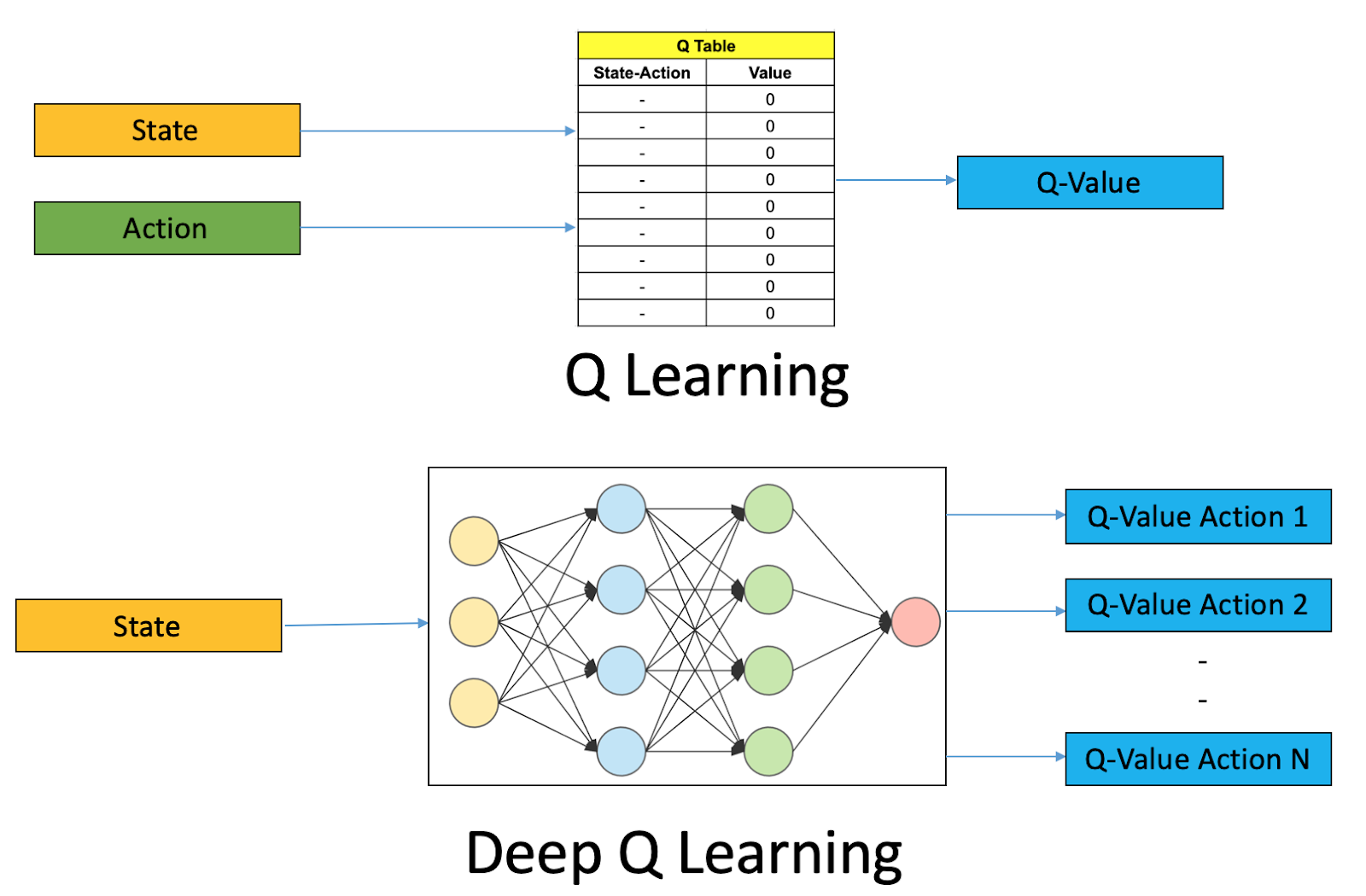
The Q-table seems feasible for problems involving smaller discrete states. As the actions and states grow, a Q-table isn’t a viable option. We need an approximate function that maps states and actions. At every time step, the agent has to compute the predicted value from the state-action approximation. This again is infeasible if the state-action pair is non-linear and discontinuous.
A Deep Artificial Neural Network (represented by $Q(S,a;\theta)$, where theta corresponds to the trainable weights of the network) could be utilized in such scenarios. A Neural Network can represent complex state spaces lucidly. Here’s an illustration:
The DQN cost function looks like:
$$Cost=[Q(S,a;\theta) - (r(S, a) + D.max_{a}Q(S^{'},a;\theta))]^2$$
It is the mean squared error (MSE) between the current $Q$ value (expected future reward) and the immediate and future rewards (actual rewards).
Training Process: The training dataset keeps building throughout the training process. We ask the agent to select the best action using the current network. The state, action, reward, and the next state are all recorded (new training data samples). The memory buffers used in such networks are typically known as Experience Replay. They break the correlation between consecutive samples which would otherwise have led to inefficient training.
Conclusion
Reinforcement Learning is a branch of Machine Learning that's aimed at automated decision-making. Its capability to analyze and replicate human intelligence has created new pathways in AI research. Understanding its significance is a necessity, with more and more research institutes and companies focusing on deploying agents for intelligent decision-making.
In this article, you've gained an understanding of what Reinforcement Learning constitutes. Put your knowledge together by building an end-to-end RL solution to a problem. Getting started with OpenAI Gym is a good place to begin (and includes a detailed Gradient Community Notebook with full Python code, free to run).