Building a Checkers Gaming Agent Using Deep Q-Learning

One of the most intriguing learning methods in machine learning literature is reinforcement learning. Through reward and punishment, an agent learns to reach a given goal by selecting an action from a set of actions in a known or unknown environment. Reinforcement learning, unlike supervised and unsupervised learning techniques, does not require any initial data.

In this article, we will demonstrate how to implement a version of the reinforcement learning technique Deep Q-Learning, to create an AI agent capable of playing Checkers at a decent level.

Introduction to Deep Q-Learning

Deep reinforcement learning is a branch of machine learning that combines deep learning and reinforcement learning (RL). RL takes into account the challenge of having a computational agent learn by making mistakes. Because deep learning is incorporated into the solution, agents can make decisions based on input from unstructured data without having to manually engineer the state space. Deep RL algorithms are able to process enormous amounts of data and determine the best course of action to take in order to achieve an objective: winning a checkers game for example.

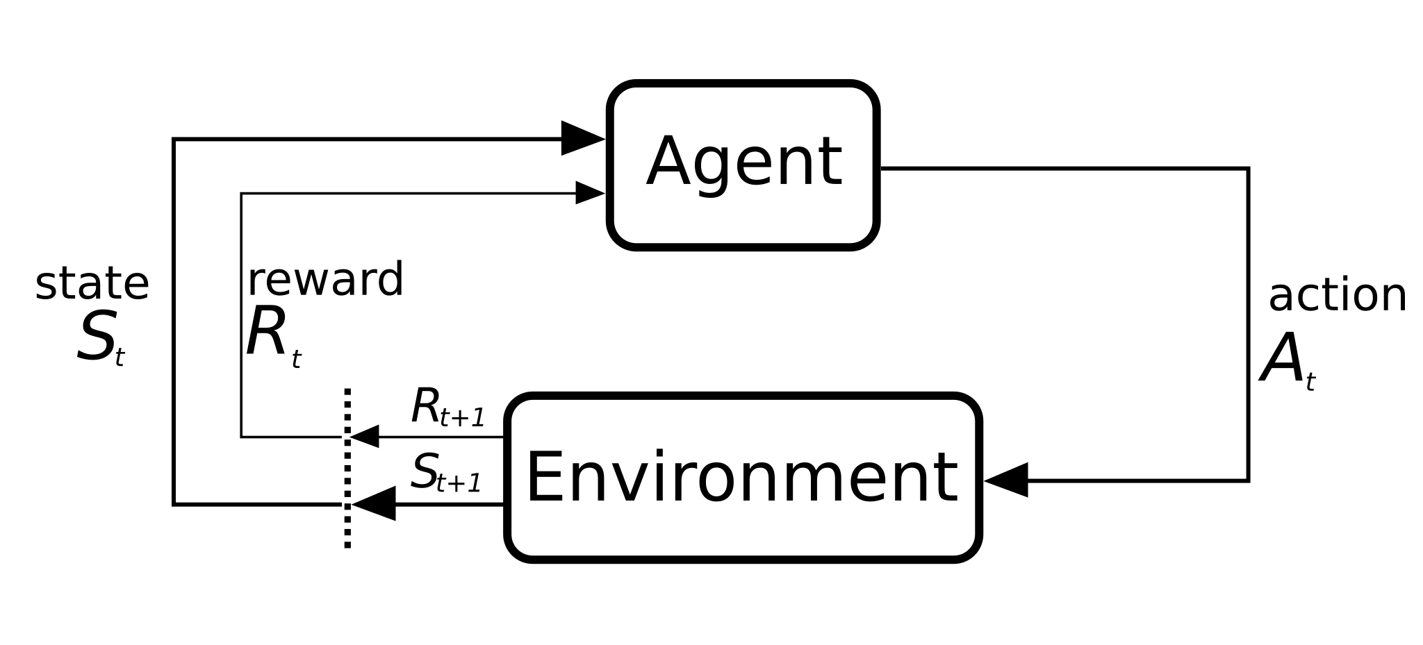
First, let's discuss what distinguishes reinforcement learning from supervised or unsupervised learning. It's basically two elements: The environment and the agent.

In a deep reinforcement learning task, an agent that interacts with its environment is being trained. The agent performs actions to reach various scenarios, or states. Rewards for actions can be both positive and negative.
The agent's sole goal in this situation is to maximize its overall reward for the entire episode. This episode (also called generation) includes everything that occurs in the environment between the initial state and the final state.

There is now a set of actions that must be completed in order to win and receive a positive reward. The concept of delayed reward comes into play here. The key to RL is learning to execute these sequences while maximizing the reward at each generation, to finally reach a winning state. This is called the Markov Decision Process.

Let’s take the example of the checkers game:

• The player is the agent interacting with the environment
• The states can be expressed as the matrix of the checkers board with each pawn and king position
• An episode/generation can represent a number of played games.
• The actions are moving pieces that can be moved and capturing opponent pieces that can be captured.
• The outcomes of these actions are used to define rewards. If the action brings the player closer to a win, a positive reward should be given; otherwise, a negative reward should be assigned.

Deep Q-Learning is unique in that we use this reinforcement learning technique to update the weight of a neural network. This is accomplished by assigning a quantifiable value to each set of (action, state), which is known as the Q-Value. Then, for each generation, we update this Q-Value to maximize the rewards.

This process of Q-value update is done using the Bellman equation, using the weighted average of the old value and the new information:

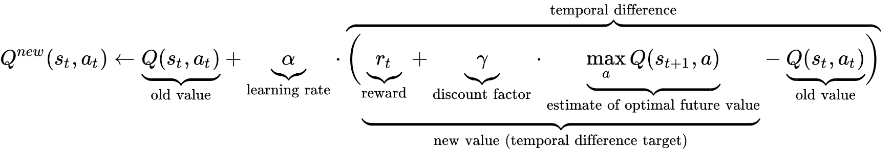
Being at the core of Deep Q-Learning, this equation introduces some significant quantities that require attention:

• Learning rate: The learning rate affects how much freshly learned knowledge supersedes previously learned information. A factor of 0 causes the agent to learn nothing, but a factor of 1 causes the agent to only take into account the most recent information, ignoring the agent's prior knowledge. In practice, a low, fixed learning rate, like 0.2, is frequently employed.
• Discount factor: The significance of future rewards is determined by the discount factor. A number close to 1 will cause the agent to seek for a long-term high payoff, while a value close to 0 will cause it to be short-sighted by only considering immediate rewards. For our case, a high value of discount factor should be implemented, because winning the game is much more important than having an intermediate "good" position.
• Initial Q-Value: Q-learning assumes an initial state before the first update because it is an iterative method. High starting values can promote exploration because the update rule will always make the chosen action have lower values than the alternatives, increasing the likelihood that they will choose it.
  To avoid divergence, it is always best to choose the initial value based on some logic and avoid randomness. This can be accomplished through previous experiences (such as expert games of checkers or chess) or by generating some "fake" experiences using a given logic (for example, evaluation of checkers positions according to predefined set of rules).

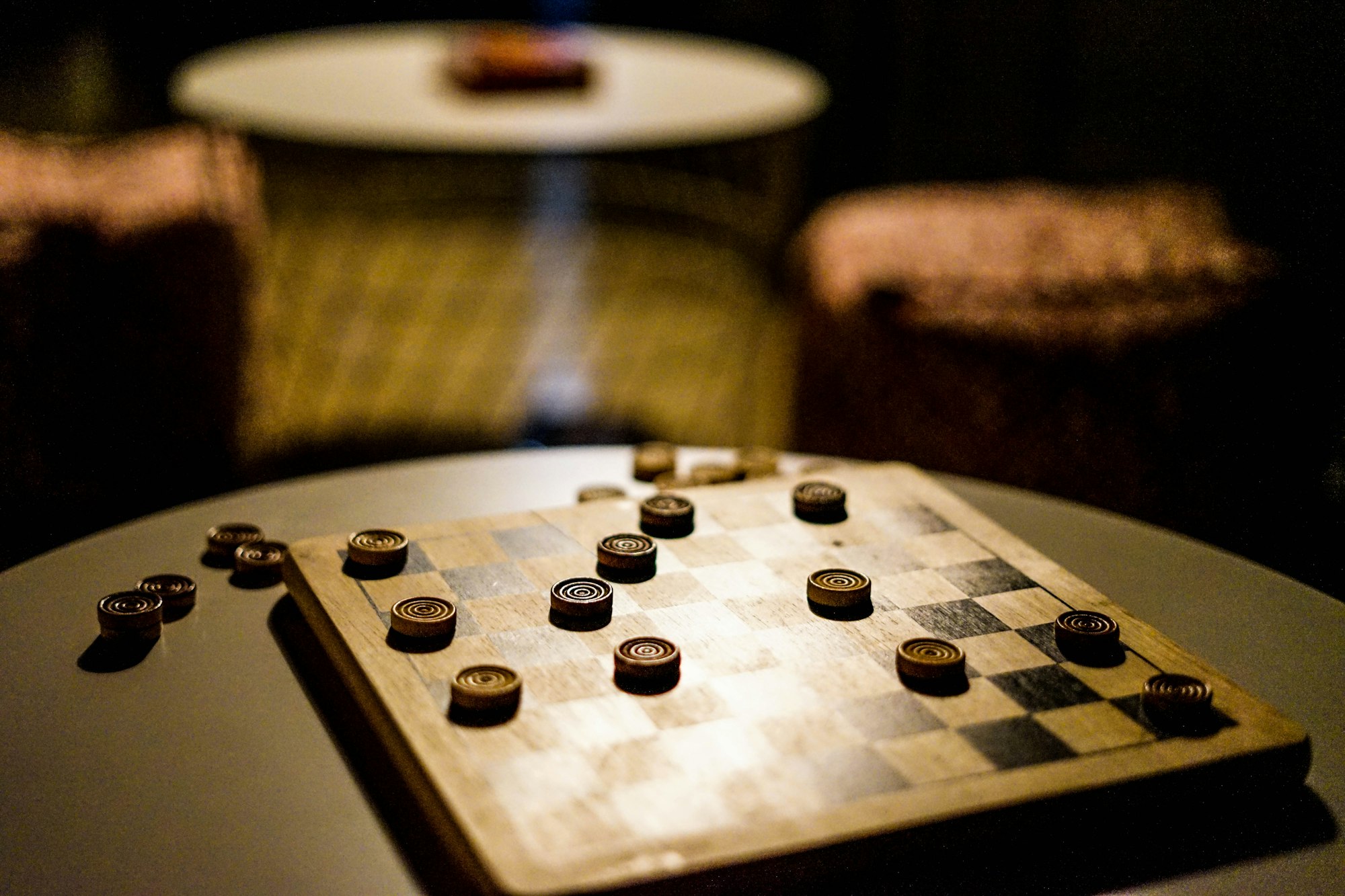
Checkers game

Being one of the most know board games, checkers is present under different variants. We counted at least 25 variant in the official wikipedia article. In this tutorial, we will be implementing the standard 8x8 American checkers with 12 initial pawns.

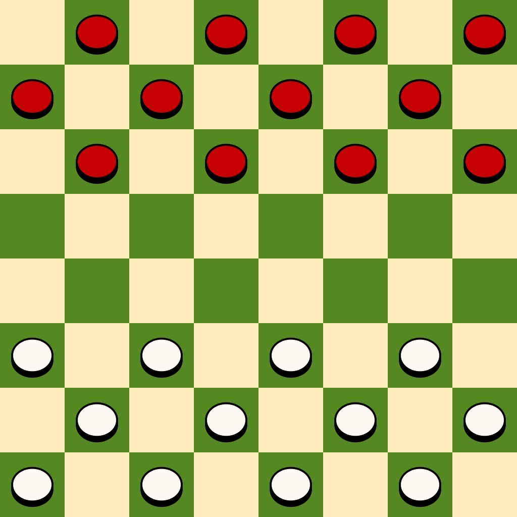
This version of checkers, also called English draughts, can be considered as the most basic. It uses a rule of No flying kings where pawns cannot capture backwards. We suggest this article for the full list of rules.

Mathematically, the game can be modeled using an 8-by-8 matrix, with a value representing the content of each cell : occupied by player 1, occupied by player 2, empty cell or unreachable cell. However, a more compress version can also be used: we can implement an 8-by-4 matrix (or a 32-by-1 array) by neglecting the unreachable cells since they never change the value during the game.

For this, we will modify a publicly available library. This library contains all the needed functions for playing the game: possible moves, possible captures, generating next position, check the game winner, and many other useful functions.

!wget "https://raw.githubusercontent.com/adilmrk/checkers/main/checkers.py"

This library introduces a critical function called get_metrics, which should be thoroughly examined.

def get_metrics(board): # returns [label, 10 labeling metrics]
	b = expand(board)

	capped = num_captured(b)
	potential = possible_moves(b) - possible_moves(reverse(b))
	men = num_men(b) - num_men(-b)
	kings = num_kings(b) - num_kings(-b)
	caps = capturables(b) - capturables(reverse(b))
	semicaps = semicapturables(b)
	uncaps = uncapturables(b) - uncapturables(reverse(b))
	mid = at_middle(b) - at_middle(-b)
	far = at_enemy(b) - at_enemy(reverse(b))
	won = game_winner(b)

	score = 4*capped + potential + men + 3*kings + caps + 2*semicaps + 3*uncaps + 2*mid + 3*far + 100*won
	if (score < 0):
		return np.array([-1, capped, potential, men, kings, caps, semicaps, uncaps, mid, far, won])
	else:
		return np.array([1, capped, potential, men, kings, caps, semicaps, uncaps, mid, far, won])

This function evaluates a given board state, based on many parameters that can give us a gross idea on which player have a better position. This will be extremely useful for creating the initial model that we will later reinforce via the Deep Q-Learning.

The Metrics model

Generative models are a subset of statistical models that produce new data instances. Unsupervised learning use these models to carry out tasks including estimating probability and likelihood, modeling data points, and classifying entities using these probabilities.

In our case, we will implement a generative model that takes as input an array of metrics (measured by the function get_metrics), then predicts the winning probability. So, this model will only looks at the 10 heuristic scoring metrics for labeling. Then later in the board model, we will use the metrics model to create a different model that directly takes as input the board as a 32 integer array and produce an evaluation of the board.

For this, we will implement a basic Sequential Keras Model, with three dense layers, a Rectified Linear Unit as an activation function and an input with size 10 representing the measured scoring metrics.

# Metrics model, which only looks at heuristic scoring metrics used for labeling
metrics_model = Sequential()
metrics_model.add(Dense(32, activation='relu', input_dim=10)) 
metrics_model.add(Dense(16, activation='relu',  kernel_regularizer=regularizers.l2(0.1)))

# output is passed to relu() because labels are binary
metrics_model.add(Dense(1, activation='relu',  kernel_regularizer=regularizers.l2(0.1)))
metrics_model.compile(optimizer='nadam', loss='binary_crossentropy', metrics=["acc"])

start_board = checkers.expand(checkers.np_board())
boards_list = checkers.generate_next(start_board)
branching_position = 0
nmbr_generated_game = 10000
while len(boards_list) < nmbr_generated_game:
	temp = len(boards_list) - 1
	for i in range(branching_position, len(boards_list)):
		if (checkers.possible_moves(checkers.reverse(checkers.expand(boards_list[i]))) > 0):
				boards_list = np.vstack((boards_list, checkers.generate_next(checkers.reverse(checkers.expand(boards_list[i])))))
	branching_position = temp

# calculate/save heuristic metrics for each game state
metrics	= np.zeros((0, 10))
winning = np.zeros((0, 1))

for board in boards_list[:nmbr_generated_game]:
	temp = checkers.get_metrics(board)
	metrics = np.vstack((metrics, temp[1:]))
	winning  = np.vstack((winning, temp[0]))
 
# fit the metrics model
history = metrics_model.fit(metrics , winning, epochs=32, batch_size=64, verbose=0)

After establishing the model, we produced 10000 games using a tree exploration starting from a specific board. The heuristic metrics were then calculated for each game. Finally, we trained the algorithm to predict the game's outcome based on these data.

The training processing history is then plotted using Matplotlib

# History for accuracy
plot.plot(history.history['acc'])
plot.plot(history.history['val_acc'])
plot.title('model accuracy')
plot.ylabel('accuracy')
plot.xlabel('epoch')
plot.legend(['train', 'validation'], loc='upper left')
plot.show()

# History for loss
plot.plot(history.history['loss'])
plot.plot(history.history['val_loss'])
plot.title('model loss')
plot.ylabel('loss')
plot.xlabel('epoch')
plot.legend(['train', 'validation'], loc='upper left')
plot.show()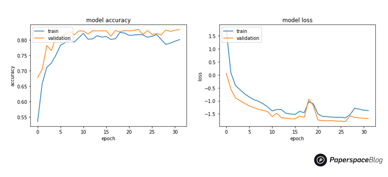

The Board model

Next, we use the metrics model to create a new one that takes an input the compressed version of the board (size 32) and predicts the probability of winning from the given board. In other words, it evaluates the position: a negative evaluation will probably lead to a losing game, and a positive one will probably lead to a winning game.

This position evaluation concept is the same concept applied to AI engines for playing the major board games: Chess, Go and other variations of Checkers.

# Board model
board_model = Sequential()

# input dimensions is 32 board position values
board_model.add(Dense(64 , activation='relu', input_dim=32))

# use regularizers, to prevent fitting noisy labels
board_model.add(Dense(32 , activation='relu', kernel_regularizer=regularizers.l2(0.01)))
board_model.add(Dense(16 , activation='relu', kernel_regularizer=regularizers.l2(0.01))) # 16
board_model.add(Dense(8 , activation='relu', kernel_regularizer=regularizers.l2(0.01))) # 8

# output isn't squashed, because it might lose information
board_model.add(Dense(1 , activation='linear', kernel_regularizer=regularizers.l2(0.01)))
board_model.compile(optimizer='nadam', loss='binary_crossentropy')

# calculate heuristic metric for data
metrics = np.zeros((0, 10))
winning = np.zeros((0, 1))
data = boards_list

After compiling the model, we will loop through all the generated board positions. And, for each board we extract the metrics, then use the metrics model to predict the probability of winning from this board.

We also calculate a confidence level for each board evaluation:

The confidence values are used as sample weight for the Keras model, to emphasize the evaluations with higher probabilities.

for board in data:
	temp = checkers.get_metrics(board)
	metrics = np.vstack((metrics, temp[1:]))
	winning = np.zeros((0, 1))
 
# calculate probilistic (noisy) labels
probabilistic = metrics_model.predict_on_batch(metrics)

# fit labels to {-1, 1}
probabilistic = np.sign(probabilistic)

# calculate confidence score for each probabilistic label using error between probabilistic and weak label
confidence = 1/(1 + np.absolute(winning - probabilistic[:, 0]))
 
# pass to the Board model
board_model.fit(data, probabilistic, epochs=32, batch_size=64, sample_weight=confidence, verbose=0)

board_json = board_model.to_json()
with open('board_model.json', 'w') as json_file:
	json_file.write(board_json)
board_model.save_weights('board_model.h5')

print('Checkers Board Model saved to: board_model.json/h5')

After fitting the model, we save weight and the model configuration to json and h5 files, that we will later use for the reinforcement learning.

We now have a model that represents a beginner level of checker expertise; the output of this model represents our initial Q-Value. Using this method to generate an initial Q-Value will make reinforcement learning considerably more efficient, because the trained board model is much better at evaluating board position than the alternative, which is randomly selecting an evaluation.

Reinforcing the model

Now that the initial model is trained, we will use Deep Q-Learning to guide it through generating more wins and draws and less losses.

In our case, we will use the concept of delayed reward. We will, go through 500 generations during the reinforcement of our model, where each generation will represent a refitting of the model. In each of these generations, the agent (model for playing the checkers) will play 200 games. And, for each game, all moves that led it to lose the game will have a negative reward, and all the ones that led to a win or a draw will get a positive reward instead.

At each step, for choosing a move, we will evaluate, using the model, all the possible moves and chose the one with the highest evaluation.

After setting the reward value at the end of each game, we will update the Q-Value using the Bellman equation, then save the updated version, along with all positions that led to the final result, until the end of the generation. Finally, at the end of each generation, the model is refitted on all the positions of these games with an updated Q-Value (evaluation).

json_file = open('board_model.json', 'r')
board_json = json_file.read()
json_file.close()

reinforced_model = model_from_json(board_json)
reinforced_model.load_weights('board_model.h5')
reinforced_model.compile(optimizer='adadelta', loss='mean_squared_error')

data = np.zeros((1, 32))
labels = np.zeros(1)
win = lose = draw = 0
winrates = []
learning_rate = 0.5
discount_factor = 0.95

for gen in range(0, 500):
	for game in range(0, 200):
		temp_data = np.zeros((1, 32))
		board = checkers.expand(checkers.np_board())
		player = np.sign(np.random.random() - 0.5)
		turn = 0
		while (True):
			moved = False
			boards = np.zeros((0, 32))
			if (player == 1):
				boards = checkers.generate_next(board)
			else:
				boards = checkers.generate_next(checkers.reverse(board))

			scores = reinforced_model.predict_on_batch(boards)
			max_index = np.argmax(scores)
			best = boards[max_index]

			if (player == 1):
				board = checkers.expand(best)
				temp_data = np.vstack((temp_data, checkers.compress(board)))
			else:
				board = checkers.reverse(checkers.expand(best))

			player = -player

			# punish losing games, reward winners  & drawish games reaching more than 200 turns
			winner = checkers.game_winner(board)
			if (winner == 1 or (winner == 0 and turn >= 200) ):
				if winner == 1:
					win = win + 1
				else:
					draw = draw + 1
				reward = 10
				old_prediction = reinforced_model.predict_on_batch(temp_data[1:])
				optimal_futur_value = np.ones(old_prediction.shape)
				temp_labels = old_prediction + learning_rate * (reward + discount_factor * optimal_futur_value - old_prediction )
				data = np.vstack((data, temp_data[1:]))
				labels = np.vstack((labels, temp_labels))
				break
			elif (winner == -1):
				lose = lose + 1
				reward = -10
				old_prediction = reinforced_model.predict_on_batch(temp_data[1:])
				optimal_futur_value = -1*np.ones(old_prediction.shape)
				temp_labels = old_prediction + learning_rate * (reward + discount_factor * optimal_futur_value - old_prediction )
				data = np.vstack((data, temp_data[1:]))
				labels = np.vstack((labels, temp_labels))
				break
			turn = turn + 1

		if ((game+1) % 200 == 0):
			reinforced_model.fit(data[1:], labels[1:], epochs=16, batch_size=256, verbose=0)
			data = np.zeros((1, 32))
			labels = np.zeros(1)
	winrate = int((win+draw)/(win+draw+lose)*100)
	winrates.append(winrate)
 
	reinforced_model.save_weights('reinforced_model.h5')
 
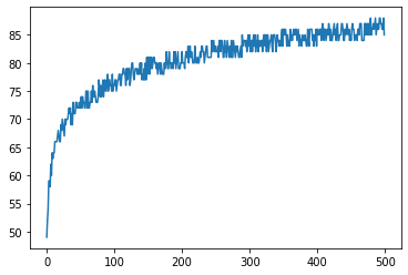
print('Checkers Board Model updated by reinforcement learning & saved to: reinforced_model.json/h5')

After running the reinforcement which can take up to few hours, where cloud AI come in handy, we plotted using matplotlib the win/draw rate values through the generations.

generations = range(0, 500)
print("Final win/draw rate : " + str(winrates[499])+"%" )
plot.plot(generations,winrates)
plot.show()

We can notice that the win/draw rate reaches a maximum of 85% by the end of the 500th generation. Which is considered as an expert level for checkers.

However, similar training techniques can be applied to have a more proficient playing agent, by also punishing the draws by assigning them negative rewards as well.

This, would probably need more number of generations and higher computing power to reinforce the model up to a decent win rate in an acceptable time.

Using the model

Now that we have a board evaluation model, the question is how to chose the best move from a given position. The basic approach is to introduce a search function that goes through all the possible moves and find the one leading to the highest evaluation.

Other strategies, such as going deeper in the search tree and exploring possible positions in more than one round, can also be used. To reach large depths (often up to 30 moves ahead), high performance chess and checker engines use approaches such as AlphaBeta Pruning, in which the search algorithm optimizes the player's possible future evaluations while minimizing the opponent's possible future evaluation.

For our case, we implemented a simple lookup function that maximizes the possible evaluation in the next turn. We also introduce a simple print function that present the board in a readable format.

def best_move(board):
  compressed_board = checkers.compress(board)
  boards = np.zeros((0, 32))
  boards = checkers.generate_next(board)
  scores = reinforced_model.predict_on_batch(boards)
  max_index = np.argmax(scores)
  best = boards[max_index]
  return best

def print_board(board):
  for row in board:
    for square in row:
      if square == 1:
        caracter = "|O"
      elif square == -1:
        caracter = "|X"
      else:
        caracter = "| "
      print(str(caracter), end='')
    print('|')

Let's test the model by predicting a move on a given position

start_board = [1, 1, 1, 1,  1, 1, 1, 0,  1, 0, 0, 1,  0, 0, 1, 0,  0, 0, 0, 0,  0, 0, -1, -1,  -1, -1, -1, -1,  -1, -1, -1, -1]
start_board = checkers.expand(start_board)
next_board = checkers.expand(best_move(start_board))

print("Starting position : ")
print_board(start_board)

print("\nBest next move : ")
print_board(next_board)

In this example, we started from a position in the middle game which is considered the hardest phase of the game.

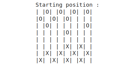
Then, using the function best_move previously introduced, we found the best next move for the player marked O, then printed the resulting board.

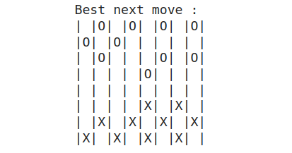
The detected move follows the basic principles of checkers that experts prescribe, which is to not leave pawns stranded in the center of the board and to back them up with back pawns as much as possible. And the model goes hand in hand with this rule.

Going Further

This tutorial's checkers engine is more than capable of defeating the ordinary casual player and even decent players. However, in order to produce an engine capable of competing with the best in the world, more severe practices must be used:

• The number of generations must be increased.
• The amount of games produced per generation must increase.
• To discover the appropriate learning rate and discount factor, some tuning strategies must be used.
• To discover the optimal move, the Alpha Beta pruning depth search technique must be used.
• We can also consider expert games as initial dataset for training the board model, instead of using the heuristic metrics.

Conclusion

In this article, we demonstrated how to use Deep Q-Learning, a type of reinforcement learning, to develop an AI agent capable of playing Checkers at a reasonable win/draw rate of 85 percent.

First, we created generative model that estimates the winning probability based on heuristic checkers metrics. Then, used it to create a board evaluation model. Next, using Deep Q-Learning, we proceeded to reinforce the board model to have more games ending with wins and draws instead of loses.

Finally, using the model we introduced, we showed how to chose from a given position, the best choice for the next move.