LLMs on DO+PS Multinode H100s: Pretraining and Finetuning MosaicML Models

We run large language model (LLM) pretraining and finetuning end-to-end using Paperspace by DigitalOcean's multinode machines with H100 GPUs. 4 nodes of H100×8 GPUs provide up to 127 petaFLOPS of compute power, enabling us to pretrain or finetune full-size state-of-the-art LLMs in just a few hours.

In this blogpost, we show how this process proceeds in practice end-to-end, and how you too can run your AI and machine learning on DigitalOcean.

In a previous post, we showed how to finetune MosaicML's MPT-7B model on a single A100-80G×8 node, walking through the process while providing some context on LLMs, data preparation, licensing, model evaluation and model deployment, alongside the usual training component.

Here, we build upon this to increase our model size to MPT-30B, add model pretraining with MPT-760m, and update our hardware from single node A100-80G×8 to multinode H100×8.

H100s on DigitalOcean

Following their launch on January 18th, Paperspace by DigitalOcean (PS by DO) now offers access to Nvidia H100 GPUs, in either H100×1 or H100×8 configurations.

This provides a number of advantageous features for the user:

• Ability to use this state-of-the-art Nvidia GPU
• Easy access to GPUs, as it was on Paperspace
• Simplicity of use via DigitalOcean's cloud
• High reliability and availability
• Ready-to-go AI/ML software stack via ML-in-a-Box
• Comprehensive and responsive customer support

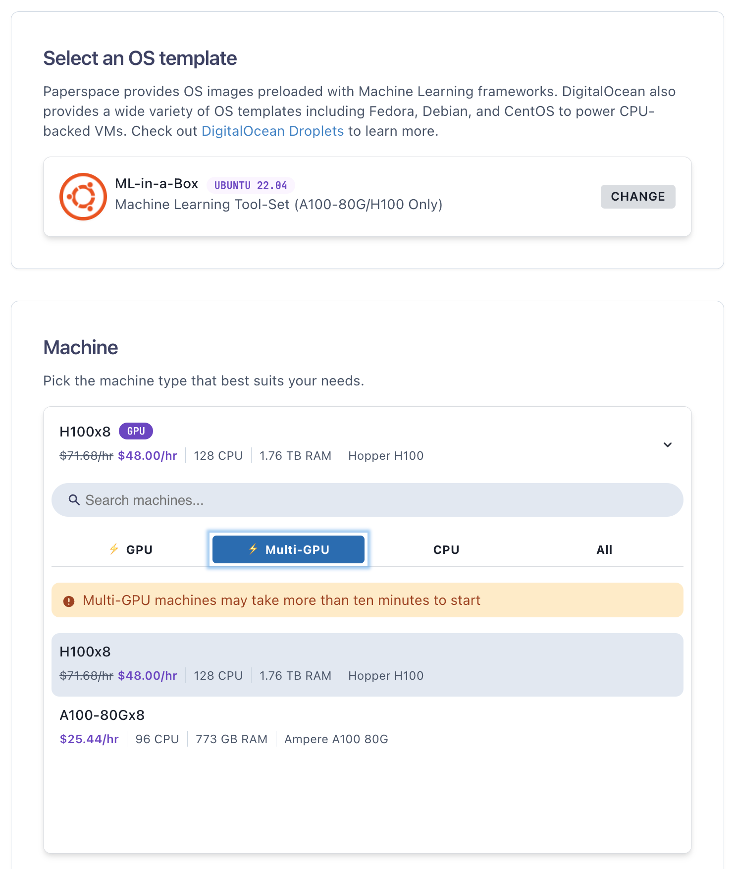
H100s can be accessed in the same way as our other GPUs, via the Paperspace GUI. Use the ML-in-a-Box template and choose H100×8:

MosaicML MPT Models

MosaicML maintains their LLM Foundry GitHub repository, where the MPT series of models is available. It continues to provide these open source LLMs in an up-to-date manner in a setup that works in practice end-to-end.

We described these models a bit more in the previous post, and here are focusing on two in particular:

• MPT-760m for pretraining: The MPT series contains models in a range of sizes, named by the number of parameters they have (m = millions, b = billions): 125m, 350m, 760m, 1b, 3b, 7b, 13b, 30b, 70b. We choose the 760m option for pretraining to provide a run of a good size, but without having to wait days or weeks for it to go through. (The larger models are not only bigger size, but also need training for more batches. 7B's original pretraining by MosaicML took 9.5 days on 440 A100-40G GPUs, at a cost of $200k.)
• MPT-30B for finetuning: often generic LLMs can respond to questions like they are continuing a chat rather than answering the question. This is not useful when the questioner is specifically looking for the answer. The MPT-30B model is tuned to better answer questions than the base model. We chose the 30 billion parameter model because (a) it represents the full size of model than most businesses will want to tune to solve their real problems, and (b) an optimized YAML is available on LLM Foundry for the 30B. The resulting model should be similar to the MPT-30B-Instruct model that is available from MosaicML on Hugging Face.

Importantly, while being open source, these models are licensed for commercial use, meaning that you can use them on DigitalOcean to help with your business.

The End-to-End Process

So are we really doing end-to-end? Well, we're not putting these models into money-making production, but we are doing most of the steps.

A modern end-to-end AI/ML process for LLMs can be thought of as a series of steps that get iterated between. We highlight the ones that we are demonstrating here, with some brief comments.

1. Business problem
2. Origination of data
3. Data collection
4. Data storage
5. Data preparation
6. Model training
7. Model conversion to inference
8. Inference/deployment
9. Deployment to production
10. Monitoring
11. Interface to get business value

The most important comment is that while we are not doing all 11 of these steps in this blogpost, they can all be done on Paperspace by DigitalOcean. Steps 1 and 2 are somewhat external to the cloud, but with our platform the infrastructure is in place to allow everything in the list to be done.

The first step, the business problem, is that we want to pretrain an LLM from scratch on our data so that we have full control, and then finetune another one to better answer questions for our customers. Step 2 is not done here because the data already exist online. For steps 3-5, we are downloading the data, which is quite large, storing it so that it is accessible in a manner performant enough to not bottleneck the H100 GPUs, and running preparation such as tokenization. Step 6 is the model pretraining or finetuning, which we are running in full via the GitHub repository's code and YAML settings. Similarly, step 7 converts the model from the checkpoint resulting from training to a more compact format suitable for deployment. (A model running inference doesn't need all the information from training such as the optimizer states, so it can be smaller.) Step 8 is then our passing of user prompts to the model and seeing its responses.

Steps 9-11, which could be done but we are not attempting here, entail first putting the model used in step 8 on an endpoint, e.g., via Paperspace Deployments. Then monitoring software such as Arize could be integrated to see the model's state while online, and whether it is behaving correctly. Finally, step 11 would be exemplified by a webapp pointing to the model that allows nontechnical users to interact with it. Many customers already use DigitalOcean for their webapps.

Setup

Now that we have previewed the end-to-end process, let's see how to achieve it.

First, we detail how to set the model up for training on Paperspace by DigitalOcean. We then follow this by the specifics of pretraining and finetuning, and finally inference + deployment.

These sections are quite long, but they realistically reflect the number of steps that need to be taken to run LLMs at scale, and that you might take when running your own.

Let's go!

Sign up for the platform

Access to the H100 GPUs for running these models as shown here requires platform signup. As part of the process, you will be guided to request approval to start up H100 machines.

Start H100 machine(s)

When starting up in the GUI (Paperspace Core), it will inform you that a private network is required. This can seem like an inconvenience to have to manually add it when all machines need it, but it is quick and easy here: just click Add Private Network, choose a name, then select it from the Select network dropdown.

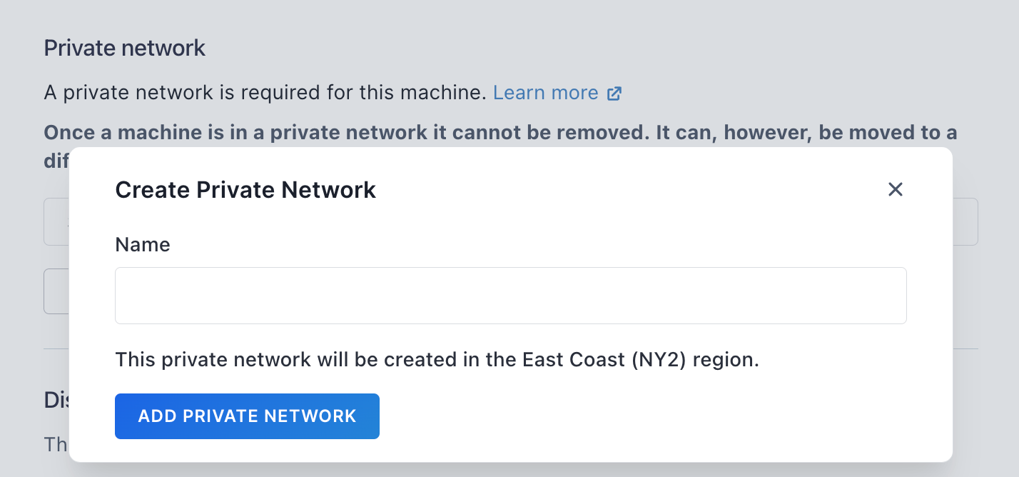
For multinode work, a private network is needed anyway for the machines to see each other. We will use it below for this purpose, and for access to a common shared drive to store our data and models.

Machine access also requires an SSH key, which is standard. The disk size should be increased from the default 100 GB, and we recommend 1-2 TB.

Other options such as dynamic IP can be left on their default settings. NVLink is enabled by default.

Access the machine from your local machine's terminal using SSH to the machine's dynamic IP, i.e., like

ssh paperspace@123.456.789.012

You can see you machine's IP from its details page in the GUI. On a Mac, iTerm2 works well, but any terminal that has SSH should work. Once accessed, you should see the machine's command line.

If you plan to do multinode work, repeat the above steps to create the number of machines (nodes) that you would like to use.

Shared drives

Paperspace's shared drives provide performant access to large files such as data and models that the user does not want to store on their machine directly, or that need to be seen across multiple machines.

Shared drives can hold up to 16 TB of data rather limit of up to 2 TB on the machine's own drive.

Setting one up requires some manual steps, but they are straightforward.

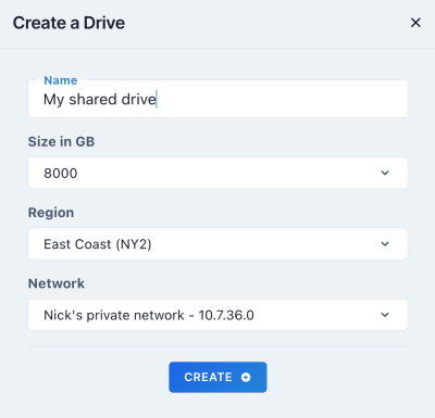
(1) In the Paperspace Core GUI, go to the Drives tab, click Create, and a modal appears with the drive details. Choose a name, size, region, and private network. The name is arbitrary, for size we recommend 2 TB or more, for region use the one under which you created your machine(s) above, and likewise for private network.

(2) From your machine's terminal, edit the /etc/fstab file to add the drive's information, so, for example

sudo vi /etc/fstab

then the credentials look like

//10.1.2.3/stu1vwx2yz /mnt/my_shared_drive cifs 
user=aBcDEfghIjKL,password=<copy from GUI>,rw,uid=1000,gid=1000,users 0 0

which can all be seen for your drive in the GUI Drives tab.

(3) Mount the shared drive using

sudo mkdir -p /mnt/my_shared_drive
sudo chown paperspace:paperspace /mnt/my_shared_drive
mount /mnt/my_shared_drive

You can check the drive is visible using df -h, where it should show up in one of the rows of output.

The process of editing /etc/fstab and mounting the shared drive needs to be repeated on all machines if you are using multinode.

Note that in principle, the shared drive could also be in a remote location such as an object store, but we didn't explore that setup for this blogpost.

MosaicML's Docker containers

Now that we are set up with our machine(s) and shared drive, we need to set up the MosaicML LLM Foundry .

To ensure an environment that is stable and reproducible with respect to our model runs, we follow their recommendation and utilize their provided Docker images.

A choice of images is presented, and we use the one with the latest version 2 Flash Attention:

docker pull mosaicml/llm-foundry:2.1.0_cu121_flash2-latest

To run the container, we need to bind-mount the shared drive to it so that it can be seen from the container, and for multinode pass various arguments so that the full H100 GPU fabric is used:

docker run -it \
  --gpus all \
  --ipc host \
  --name <container name> \
  --network host \
  --mount type=bind,source=/mnt/my_shared_drive,\
    target=/mnt/my_shared_drive \
  --shm-size=4g \
  --ulimit memlock=-1 \
  --ulimit stack=67108864 \
  --device /dev/infiniband/:/dev/infiniband/ \
  --volume /dev/infiniband/:/dev/infiniband/ \
  --volume /sys/class/infiniband/:/sys/class/infiniband/ \
  --volume /etc/nccl/:/etc/nccl/ \
  --volume /etc/nccl.conf:/etc/nccl.conf:ro \
  <container image ID>

In this command, -it is the usual container setting to get interactivity, --gpus is because we are using Nvidia Docker (supplied with our machine's ML-in-a-Box template), --ipc and --network help the network function correctly, --mount is the bind-mount to see the shared drive as /mnt/my_shared_drive within the container, --shm-size and --ulimit ensure we have enough memory to run the models, and --device & --volume set up the GPU fabric.

You can see your container's image ID from the host machine by running docker images, and your container's name is arbitrary. We used a name containing a date, like

export CONTAINER_NAME=\
`echo mpt_pretraining_node_${NODE_RANK}_\`date +%Y-%m-%d_%H%M-%S\``

for versioning purposes, NODE_RANK being 0, 1, 2, etc., for our different nodes on the network.

If you are restarting an existing container instead of creating a new one, you can use docker start -ai <container ID>, where the container ID can be seen from docker ps -a. This should put you back in the container at the command line, the same as above when a new container was created.

A final note for the container setup is that our ML-in-a-Box template contains a configuration file for the Nvidia Collective Communications Library (NCCL) that helps everything run better with H100s and our 3.2 Tb/s node interconnect. This file is in /etc/nccl.conf and contains:

NCCL_TOPO_FILE=/etc/nccl/topo.xml
NCCL_IB_DISABLE=0
NCCL_IB_CUDA_SUPPORT=1
NCCL_IB_HCA=mlx5
NCCL_CROSS_NIC=0
NCCL_SOCKET_IFNAME=eth0
NCCL_IB_GID_INDEX=1

The file is already supplied and does not need to be modified by the user.

As with the shared drives, the process here is repeated on each node if you are running multinode.

Set up GitHub repository on the container

Once we are in the container, the code can be set up by cloning the GitHub repository and then installing it as a package. Following LLM Foundry's readme, this is:

git clone https://github.com/mosaicml/llm-foundry.git
cd llm-foundry
pip install -e ".[gpu]"

On our machines, we also first installed an editor (apt update; apt install -y vim), updated pip (pip install --upgrade pip), and recorded the version of the repository that we were using (cd llm-foundry; git rev-parse main).

There are also a couple of optional steps of installing XFormers and FP8 (8-bit datatype) support for H100s: pip install xformers and pip install flash-attn==1.0.7 --no-build-isolation along with pip install git+https://github.com/NVIDIA/TransformerEngine.git@v0.10. We actually generated our results without these, but they are available as a potential optimization.

Bookkeeping

The repository works by providing Python scripts that in turn call the code to prepare the data, train the models, and run inference. In principle it is therefore simple to run, but we do need a few more steps to run things at scale in a minimally organized fashion:

• Create some directories: data, model checkpoints, models for inference, YAML files, logs, subdirectories for each node, the pretraining or finetuning tasks, various runs, and any others such as a files with prompt text
• Enable Weights & Biases logging: not strictly required, or one could integrate other libraries like TensorBoard, but this auto-plots a sample of useful metrics that give information on our runs. These include GPU usage and model performance while training. This requires a Weights & Biases account.
• Environment variables: Also not strictly required, but useful. NCCL_DEBUG=INFO was needed less as the new infrastructure become more reliable pre-launch, but we still set it. If using Weights and Biases logging, WANDB_API_KEY is required to be set to the value of your API key from there to enable logging without a manual interactive step. We set some others as well to simplify commands referring to assorted directories on multinode, and they can be seen below.

For a multinode run to do the pretraining and finetuning that we show here, a minimal set of directories is

/llm-own/logs/pretrain/single_node/
/llm-own/logs/finetune/multinode/

/llm-own/logs/convert_dataset/c4/
$SD/data/c4/

$SD/yamls/pretrain/
$SD/yamls/finetune/

$SD/pretrain/single_node/node0/mpt-760m/checkpoints/
$SD/pretrain/single_node/node0/mpt-760m/hf_for_inference/

$SD/finetune/multinode/mpt-30b-instruct/checkpoints/
$SD/finetune/multinode/mpt-30b-instruct/hf_for_inference/

where SD is the location of our shared drive, NODE_RANK is 0, 1, 2, etc., for our different H100×8 nodes. /llm-own is arbitrary, being just a place on the container to place the directories.

Some of these might look quite long, but in practice we ran more models and variations than shown in this blogpost. You can use mkdir -p to create subdirectories at the same time as the parent ones.

We will see how the directories are used below.

Ready to go!

Now the setup is complete, we are ready to move on to data preparation → model training → inference + deployment.

Pretraining MPT-760m

Now that we are set up to go by following the steps in the previous section, our first run is model pretraining. This is for MPT-760m.

We ran this on both single node and multinode. Here we show the single node, and we will show multinode for finetuning MPT-30B below.

Get the data

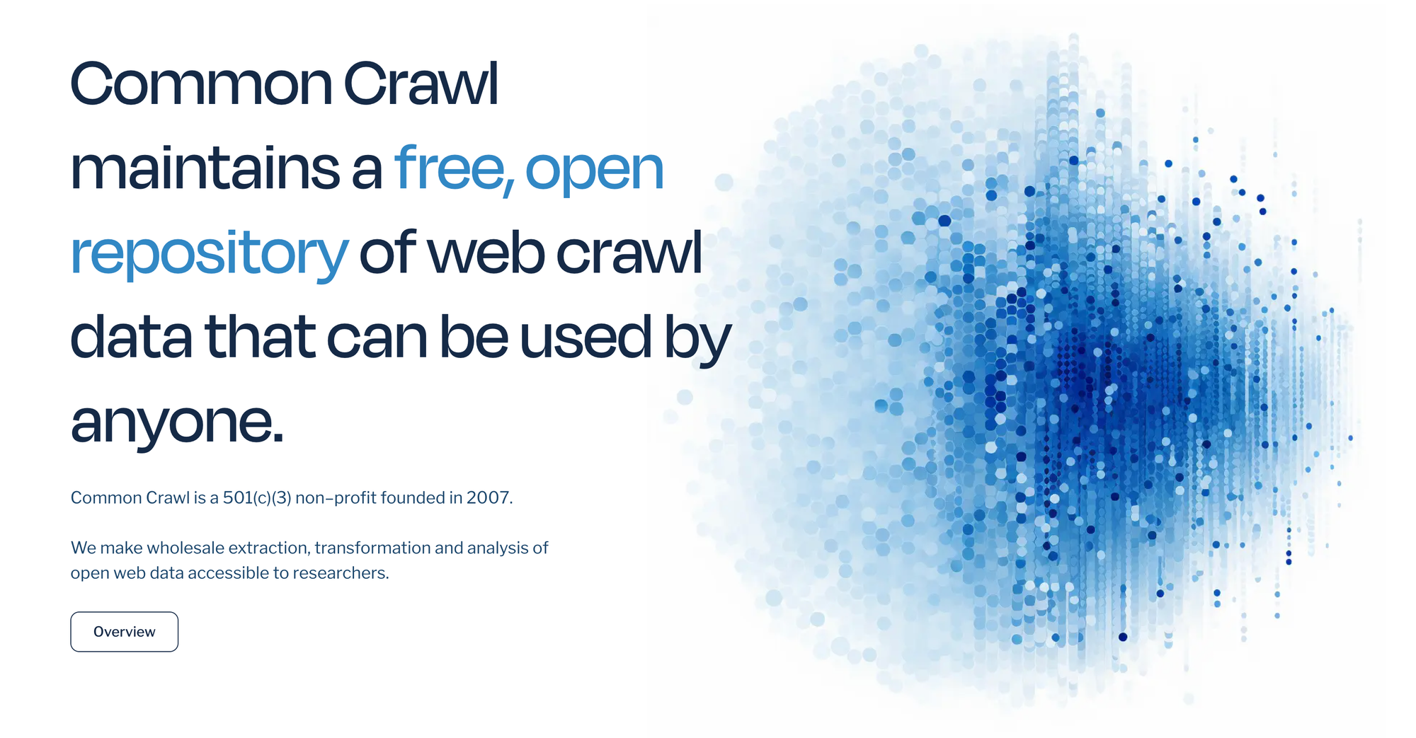
For LLM pretraining, the data are large: the C4 dataset on Hugging Face is based on the Common Crawl dataset for LLM pretraining, and contains over two million rows.

A typical row of the data looks like

{
  'url': 'https://klyq.com/beginners-bbq-class-taking-place-in-missoula/',
  'text': 'Beginners BBQ Class Taking Place in Missoula!\nDo you want to get better at making delicious BBQ? You will have the opportunity, put this on your calendar now. Thursday, September 22nd join World Class BBQ Champion, Tony Balay from Lonestar Smoke Rangers. He will be teaching a beginner level class for everyone who wants to get better with their culinary skills.\nHe will teach you everything you need to know to compete in a KCBS BBQ competition, including techniques, recipes, timelines, meat selection and trimming, plus smoker and fire information.\nThe cost to be in the class is $35 per person, and for spectators it is free. Included in the cost will be either a t-shirt or apron and you will be tasting samples of each meat that is prepared.',
  'timestamp': '2019-04-25T12:57:54Z'
}

LLM Foundry provides a script to download and prepare the data. We call it using

time python \
  /llm-foundry/scripts/data_prep/convert_dataset_hf.py \
  --dataset c4 \
  --data_subset en \
  --out_root $SD/data/c4 \
  --splits train val \
  --concat_tokens 2048 \
  --tokenizer EleutherAI/gpt-neox-20b \
  --eos_text '<|endoftext|>' \
  2>&1 | tee /llm-own/logs/convert_dataset/c4/convert_dataset_hf.log

where the command is wrapped by time ... 2>&1 tee <logfile> so we can capture the terminal stdout and stderr output to a logfile, and the wallclock time taken to run. We use this simple time ... tee wrapper throughout our work here, but it is optional.

The preprocessing doesn't use multinode or GPU, but with a good network speed for download it runs in about 2-3 hours as a one-off step, so optimizing this step onto GPU with something like DALI or GPUDirect is not important.

The script converts the downloaded data into the MosaicML StreamingDataset format, which is designed to run better when used with distributed models at scale. The resulting set of files is 20850 shards in /mnt/my_shared_drive/data/c4/train/shard.{00000…20849}.mds, plus a JSON index, and 21 shards as a validation set in val/. The total size on disk is about 1.3 TB.

YAML files

With the data available, we need to set all of the parameters describing the model and its training to the correct values. Fortunately (again), the repository has a range of these already set for both pretraining and finetuning. They are supplied as YAML files.

For the MPT-760m model, we use the values in this YAML, and leave them on the defaults except for:

data_local: /mnt/my_shared_drive/data/c4
loggers:
  wandb: {}
save_folder: /llm-own/nick_mpt_8t/pretrain/single_node/node0/\
  mpt-760m/checkpoints/{run_name}

We point to the data on the shared drive, uncomment the Weights & Biases logging, and save the model to a directory containing the run name. The name is set by the environment variable RUN_NAME, which the YAML picks up by default. We give this a date in a similar manner to the container name above for versioning purposes.

Running on a single node allows us to leave the default saving of checkpoints to save_folder every 1000 batches as-is, since they are not particularly large for the 760m model. We save them to the machine's drive to avoid an issue with symbolic linking on the shared drive — see the finetuning MPT-30B section below. They could be moved to the shared drive after the run if needed.

We talked a bit more about what many of the other YAML parameters for these models mean in the previous MPT blogpost, in its Fine-tuning run section for MPT-7B.

Run pretraining

With the data and model parameters set up, we are ready for the full pretraining run:

time composer \
  /llm-foundry/scripts/train/train.py \
  /llm-own/yamls/pretrain/mpt-760m_single_node.yaml \
  2>&1 | tee /llm-own/logs/pretrain/single_node/\
  {$RUN_NAME}_run_pretraining.log

This command uses MosaicML's composer wrapper to PyTorch, which in turn uses all 8 H100 GPUs on this node. Arguments can be passed to the command, but we have encapsulated them all in the mpt-760m_single_node.yaml YAML file.

As above, the time ... tee wrapper is ours, and is optional, so the command has in principle reduced to the very simple composer train.py <YAML file>.

Results from running pretraining

Using one H100×8 node, full MPT-760m pretraining completes in about 10.5 hours. (And on 2 nodes multinode, it completes in under 6 hours.)

We can see some aspects of the training by viewing Weights & Biases's auto-generated plots.

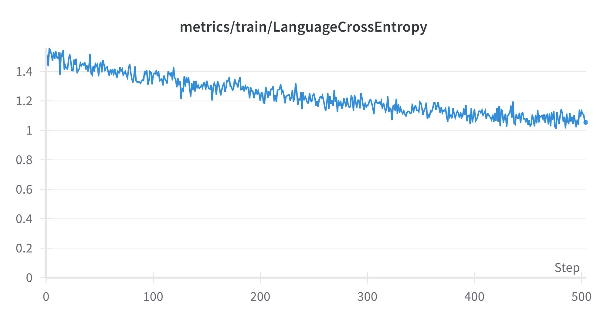
The improving model performance while training can be measured in various ways, here by default they are loss, cross-entropy, and perplexity. For cross-entropy, we see its value versus the number of batches reached in training, from 0-29000:

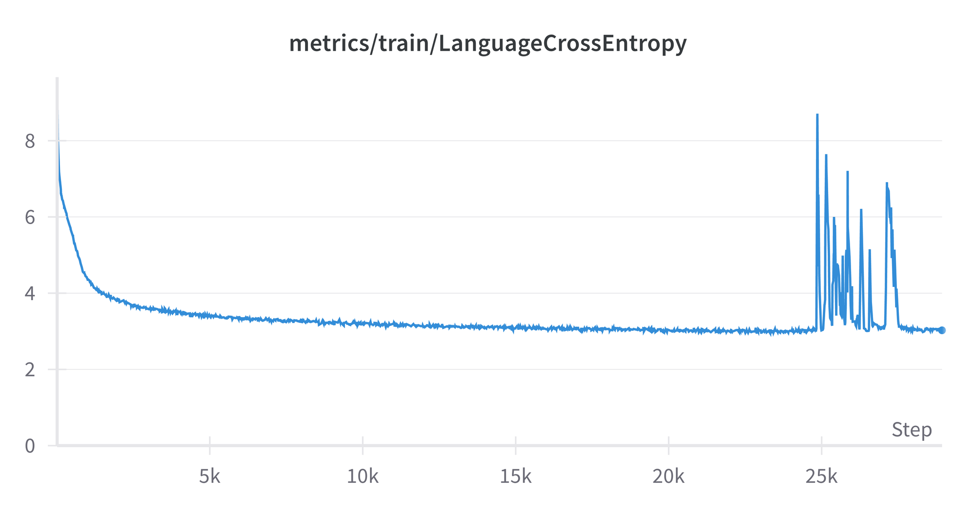
The spikes from around 25k-28k are curious, but don’t appear to affect the final result, which reflects the general flattening out of the curve around a value of 3. The plots for loss and perplexity are similar in shape, as are the ones from the model run on the evaluation set.

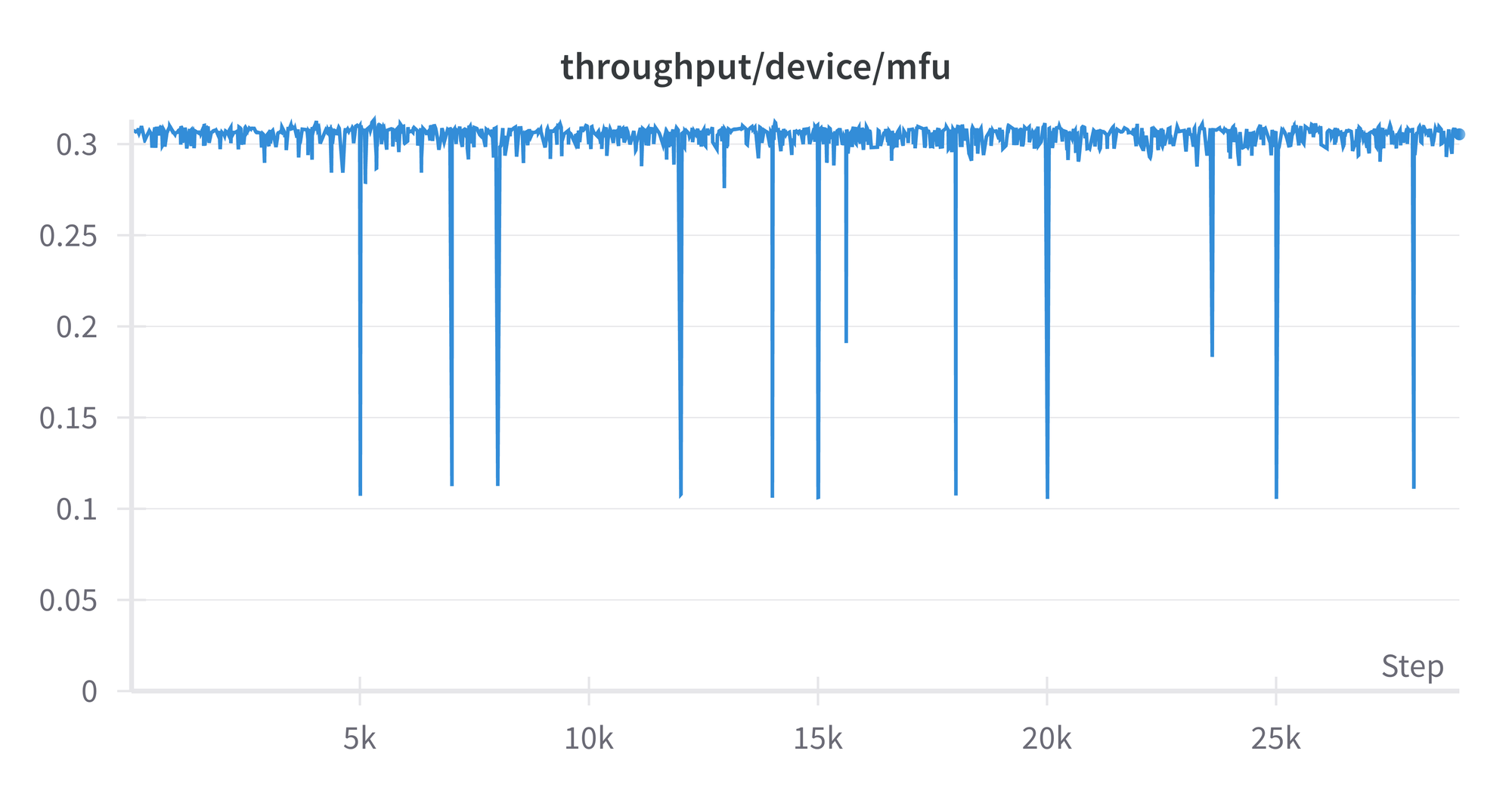
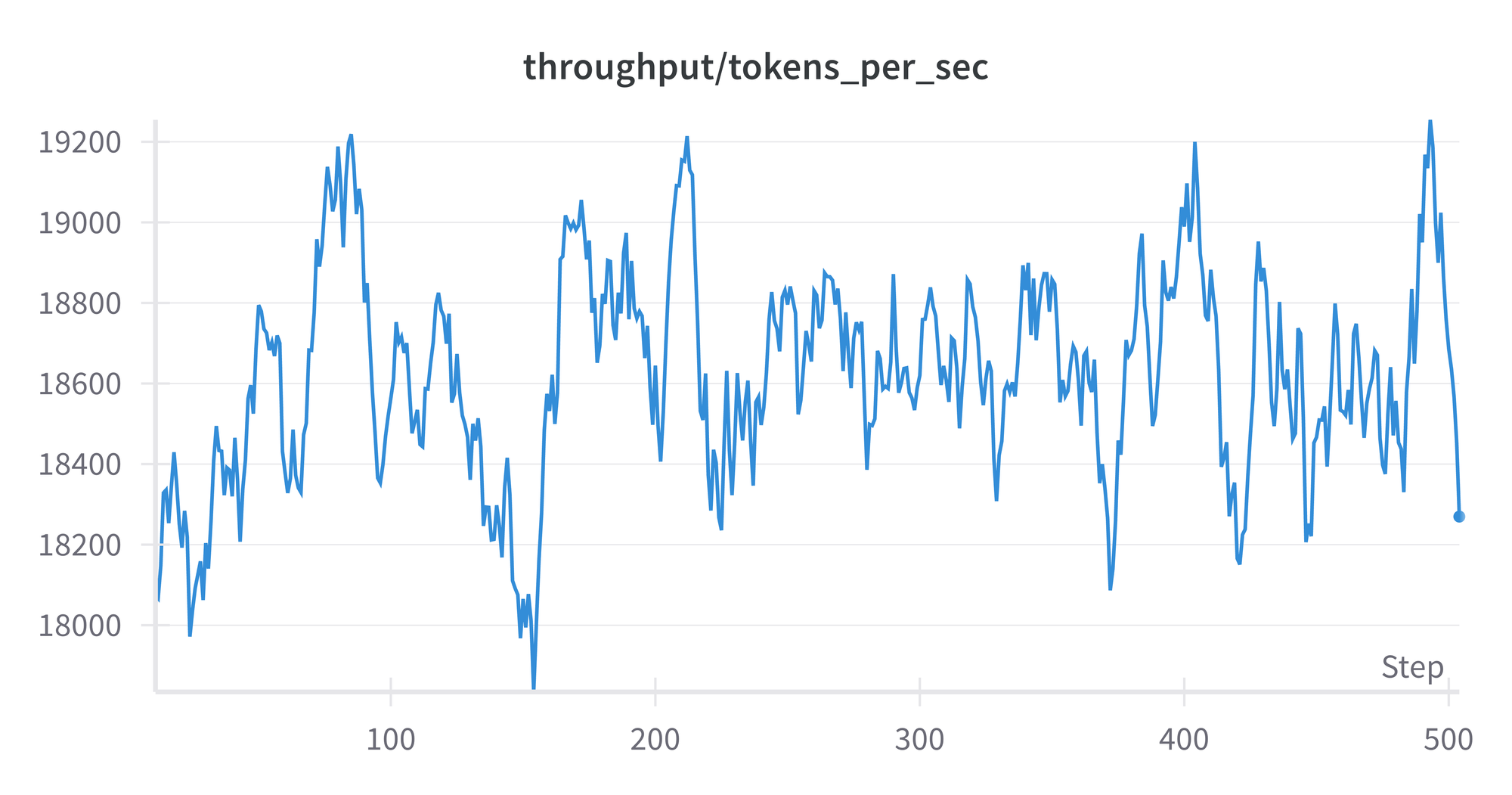
The model FLOPS utilization (MFU) shows how efficiently the GPU is being used. We see that it is stable throughout, aside from some occasional dips, and is just over 0.3. The theoretical perfect value is 1, and in practice highly optimized runs can get around 0.5. So there may be some room for improvement in our model's detailed settings, but it is not orders of magnitude off. A plot of throughput in tokens per second looks similar, around 4.5e+5.

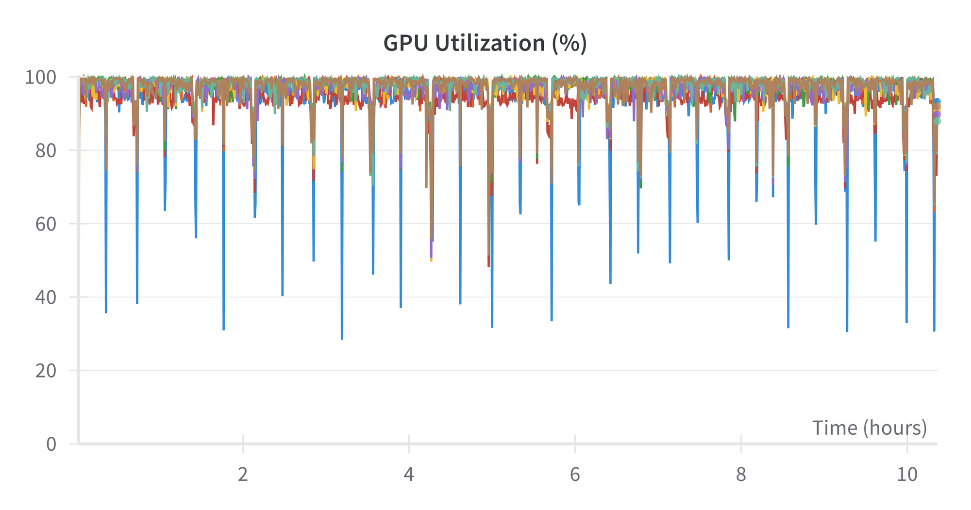
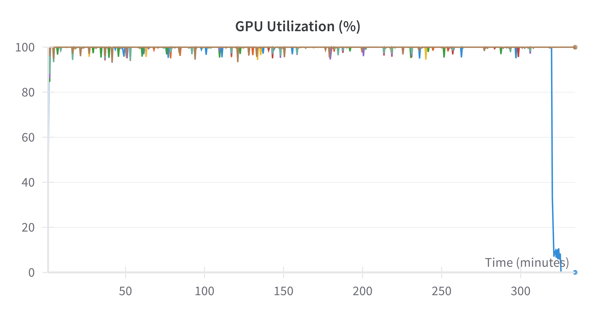
Utilization of the GPU is close to 100% throughout. The largest (blue) spikes downward are the first GPU of the 8.

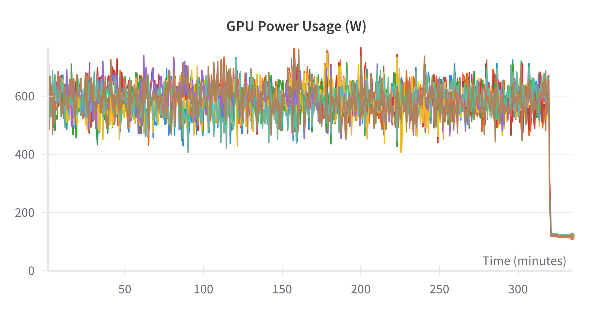
Finally, the power usage of the H100s is about 625 watts:

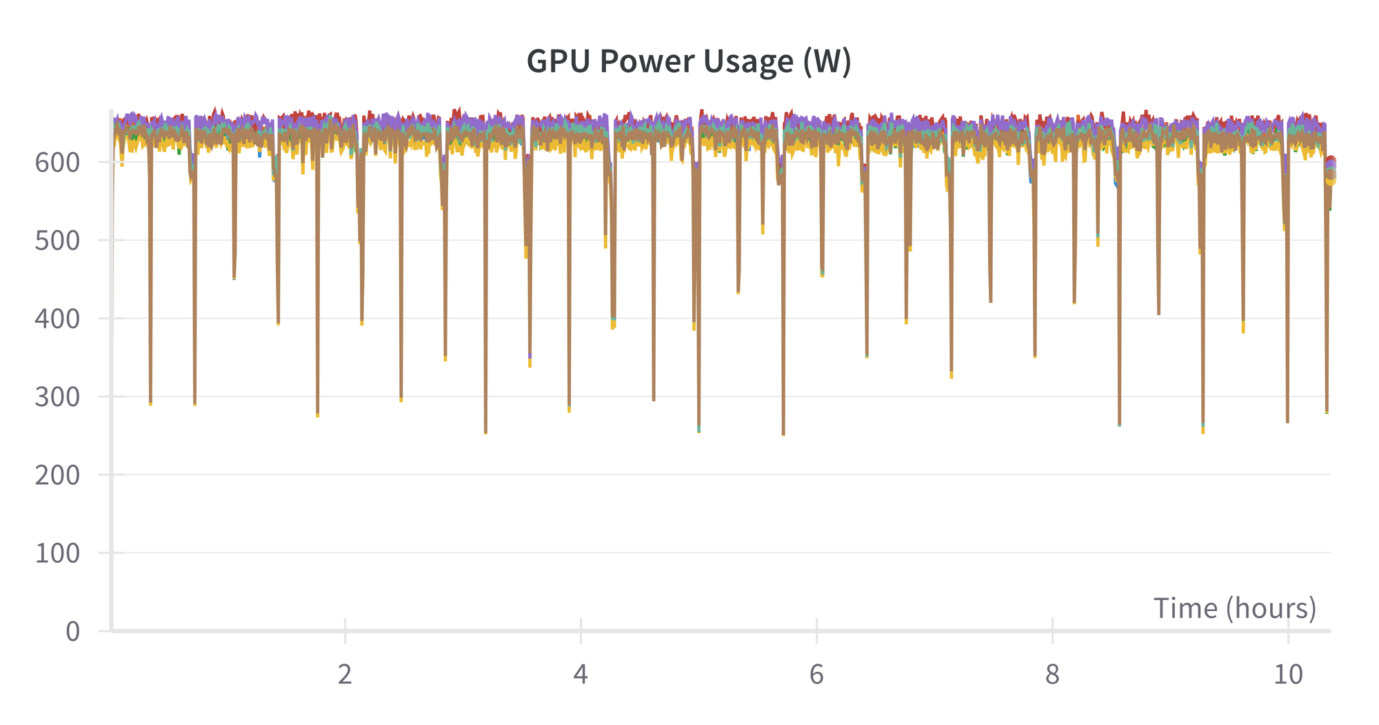
This means that the total power used for this run is about 625 watts × 10.5 hours × 8 GPUs × 1 node ~ 50 kWh

When the training is complete, the checkpoint size of the fully trained model is 8.6 GB, and it is ready to be used for inference and deployment (see below).

Finetuning MPT-30B

Above, we pretrained MPT-760m on a single H100×8 node. Here, we finetune the MPT-30B model, and show the results from using 2 nodes, i.e., multinode. (It also worked on 4 nodes.)

Get the model

While data for finetuning are generally much smaller than for pretraining, the model to be used can be much larger. This is because the model is already pretrained, meaning relatively less compute is needed.

We are therefore able to upgrade from MPT-760m in full pretraining above to finetuning the MPT-30B model with its 30 billion parameters, while maintaining a runtime of a few hours.

The initial size of MPT-30B is 56 GB, and this is automatically downloaded by the finetuning script below. After finetuing, the size on disk of the final checkpoint is 335 GB.

YAML files

The LLM Foundry is set up so that finetuning works quite similarly to pretraining from the user point of view. As above, we largely use the default YAML values, this time from here, but now make these changes:

run_name: <run name>
global_train_batch_size: 96
loggers:
  wandb: {}
save_folder: /mnt/nick_mpt_8t/finetune/multinode/\
  mpt-30b-instruct/checkpoints/{run_name}
save_interval: 999ep

The logging to Weights and Biases is similar to pretraining. We give the run name in the YAML this time. The other required change is for the global train batch size to be divisible by the total number of GPUs, here 16 for 2 nodes. The value used is fairly close to the original YAML's default of 72.

Because each checkpoint now has a size of 335 GB, we now save them directly to the shared drive rather than the machine's drive. This, however, brings up an issue with symbolic linking, discussed more in the note below, which means that the save interval has to be set to a large value.

Finally, we commented out the ICL model evaluation tasks given in the original YAML, because they needed further setup. The values of loss, entropy, and perplexity on the evaluation set are still calculated during training.

Run finetuning

Finetuning is now ready to go, and is invoked by the multinode version of the composer command:

time composer \
  --world_size 16 \
  --node_rank $NODE_RANK \
  --master_addr 10.1.2.3 \
  --master_port 7501 \
  /llm-foundry/scripts/train/train.py \
  $SD/yamls/finetune/mpt-30b-instruct_multinode.yaml \
  2>&1 | tee /llm-own/logs/finetune/multinode/\
  ${RUN_NAME}_run_finetuning.log

This is convenient, as it can be given on each node, enabling multinode training without a workload manager such as Slurm, so long as the nodes can see each other and the shared drive.

The composer command is in turn calling PyTorch Distributed. In the arguments, the --world_size is the total number of GPUs, --node_rank is 0, 1, 2, etc., for each node, 0 being the master, --master_addr is the private IP of the master node (visible on the GUI machine details page), --master_port needs to be visible on each node, and we use various environment variables so that the same command can be given on each node. The YAML captures all the other settings, and is placed on the shared drive so we only have to edit it once.

The command on node 0 waits for the command to be issued on all nodes, then runs the training with the model distributed across the nodes using a fully sharded data parallel (FSDP) setup.

Results from running finetuning

The finetuning run doesn't output the model FLOPS utilization, but we can see various other metrics similar to pretraining:

At the end of the run, we have our final 335 GB checkpoint on the shared drive.

With this in place, we are ready to proceed to inference and deployment for our pretrained and finetuned models.

Inference and Deployment

Models that have been pretrained or finetuned contain extra information, such as the optimizer states, that is not needed for running inference on new unseen data.

The LLM Foundry repository therefore contains a script to convert model checkpoints from training into the smaller and more optimized Hugging Face format suitable for deployment.

Our commands for the pretrained MPT-760m and finetuned MPT-30B are:

time python \
  /llm-foundry/scripts/inference/convert_composer_to_hf.py \
  --composer_path $SD/pretrain/single_node/node$NODE_RANK/\
    mpt-760m/checkpoints/$RUN_NAME/$CHECKPOINT_NAME \
  --hf_output_path $SD/pretrain/single_node/node$NODE_RANK/\
    mpt-760m/hf_for_inference/$RUN_NAME \
  --output_precision bf16 \
  2>&1 | tee /llm-own/logs/pretrain/single_node/\
    ${RUN_NAME}_convert_to_hf.log

time python \
  /llm-foundry/scripts/inference/convert_composer_to_hf.py \
  --composer_path $SD/finetune/multinode/\
    mpt-30b-instruct/checkpoints/$RUN_NAME/$CHECKPOINT_NAME \
  --hf_output_path $SD/finetune/multinode/\
    mpt-30b-instruct/hf_for_inference/$RUN_NAME \
  --output_precision bf16 \
  2>&1 | tee /llm-own/logs/finetune/multinode/\
    ${RUN_NAME}_convert_to_hf.log

These reduce the model sizes on disk from the 8.6 GB and 335 GB of the checkpoints to 1.5 GB and 56 GB. For the case of finetuning, we see that the converted MPT-30B is the same size as the original model downloaded at the start of the process. This is because finetuning leaves the model with the same architecture but updated weights.

While the disk space taken has been reduced, it is still in fact double the above numbers, at 3 GB and 112 GB, because the converted models are output in both .bin and .safetensors format.

(We can also note in passing that the ratio of the sizes of the two models is about the same as the ratio of their number of parameters: 30 billion / 760 million ~ 40.)

After conversion, we can "deploy" the models to run inference, by passing in user input and seeing their responses using the repository's generator script:

time python \
  /llm-foundry/scripts/inference/hf_generate.py \
  --name_or_path $SD/pretrain/single_node/node$NODE_RANK/\
    mpt-760m/hf_for_inference/$RUN_NAME \
  --max_new_tokens 256 \
  --prompts \
    "The answer to life, the universe, and happiness is" \
    "Here's a quick recipe for baking chocolate chip cookies: Start by" \
    2>&1 | tee /llm-own/logs/pretrain/single_node/\
    ${RUN_NAME}_hf_generate.log

time python \
  /llm-foundry/scripts/inference/hf_generate.py \
  --name_or_path $SD/finetune/multinode/mpt-30b-instruct/\
    hf_for_inference/$RUN_NAME \
  --max_new_tokens 256 \
  --prompts \
    "The answer to life, the universe, and happiness is" \
    "Here's a quick recipe for baking chocolate chip cookies: Start by" \
    2>&1 | tee /llm-own/logs/finetune/multinode/\
    ${RUN_NAME}_hf_generate.log

The responses seem OK.

These are the ones from MPT-760m, truncated to the character limit:

#########################################################################
The answer to life, the universe, and happiness is: the only path which matters.
The book of the year has a special place in everyone's heart.
It can be said only as a metaphor.
As we look for the meaning of life and happiness, some things that come from the heart come from the mind too. Like in this case, that something which is born with the human body begins to grow, and begins to feel the way you do, your heart grow and develop, with the help of the Holy Spirit. The world of the spirit and the universe of matter, and the eternal reality which exists in all the universe and the human body, begin to grow and to grow, and at the same time grow and to develop, to develop and to develop.
This is very good news because we can come to the heart and can find our place in the cosmos, and we become a soul.
We can come to know the true, and in truth, we can reach the truth about our existence. We can come to find peace about our life, and we can find our place in the universe, and we grow.
And we can find our place in the other side, and all have the same power.
How far have the people of Earth experienced transformation, but did not know
#########################################################################
Here's a quick recipe for baking chocolate chip cookies: Start by pouring the nuts into the butter or buttermilk and water into the pan and then sprinkle with the sugars.
Put the oven rack in the lower half of the oven and spread out 2 sheets of aluminum foil about 1 cm above the pan, and then put each rectangle in the preheated oven for 10 minutes. Once done, remove the foil.
While the nuts are cooking, put 1 tsp of maple syrup in a small pan with the sliced zucchini and stir well. Cook together with the juices, stirring occasionally. The juices are a rich syrup which you may add just prior to baking.
Once the nuts are done, add 2 tsp of melted butter, and combine just before adding the flour mixture. You may need a little more than half milk if you like yours sweet.
Transfer the batter to the baking dish and bake for 40 minutes, stirring only once every 10 minutes. You may bake the cookies for about an hour after baking.
If you are using a pan with a metal rack, place the baking sheet on a high rack and pour the nuts/butter on top of the pan. The nuts will rise like a candy bar after taking a few minutes to cook on a tray.
In another bowl mix together the flour and baking powder
#########################################################################

How to quantify exactly how good an LLM's response is to a user prompt is still a research problem. So the fact that the responses "seem OK", while appearing to be a rather cursory check, is in fact a good empirical verification that our end-to-end process has worked correctly.

We are now done running our models!

Refinements?

Our main aim here has been to demonstrate multinode LLMs working end-to-end in a way that would be satisfactory for our users to see when using Paperspace by DigitalOcean themselves. Various issues, resolutions, internal feedback, and iterative product improvements also resulted from this, but are not shown here.

There remain many refinements that could be made to future AI work at scale, both specific to this case, and more generally:

• Use XFormers and FP8: These optional installs mentioned in the setup section above may provide some extra speedup.
• Detail YAML optimization: The optimal batch size may be slightly different for H100s compared to the GitHub repository defaults.
• Fewer manual steps: Various steps here could be automated, such as passing running the same container setup followed by commands on each node.
• Symlinks: Fixing the shared drive symlink issue would make working with checkpoints more convenient.
• More prompts and responses: We only briefly used the end-result models here, checking that a few responses made sense. Checking more would be prudent for production work, for example, empirical comparison to the outputs from the baseline models, and suitability + safety of the models' responses for users.

Conclusions and next steps

We have shown that pretraining and finetuning of realistic large language models (LLMs) can be run on Paperspace by DigitalOcean (PS by DO), using single or multiple H100×8 GPU nodes.

The end-to-end examples shown are realistic and not idealized on the product as-is, and so can be used as a basis for your own work with AI and machine learning.

The combination of accessibility, simplicity of use, choice of GPUs, reliability & scale, and comprehensive customer support make PS by DO an ideal choice for businesses and other customers who want to pursue AI, whether by pretraining, finetuning, or deploying existing models.

As well as the LLMs shown here, models in other common AI fields, such as computer vision and recommender systems, are equally feasible end-to-end.

Some next steps to take are:

• Use PS by DO H100s: Sign up for PS by DO, and you will have access to the types of hardware, machines, and software used in this blogpost.
• Check out the documentation: Deep Learning with ML in a Box and NVIDIA H100 Tensor Core GPU are useful.
• Deploy models and webapps: Paperspace Deployments allows the trained models seen here running inference to be deployed to an endpoint, that can in turn be accessed by a webapp or other interface. DigitalOcean has a wide range of customers already using webapps, so it is a natural fit to use them for AI too.
• Finetune models: We have seen that the computing power, reliability & scale, software stack, and tractability exist on PS by DO to enable users who need to finetune their own models to do so.
• Solve your business (or other) problem with AI: the infrastructure presented is generic, so whether you need to use LLMs, computer vision, recommender systems, or another part of AI/ML, PS by DO is ready.

An interesting final thought is that, even after finetuning, the original model page for MPT-30B-Instruct states:

MPT-30B-Instruct can produce factually incorrect output, and should not be relied on to produce factually accurate information. MPT-30B-Instruct was trained on various public datasets. While great efforts have been taken to clean the pretraining data, it is possible that this model could generate lewd, biased or otherwise offensive outputs.

So, returning to the original business problem, it still seems that it would be more suited for recreational conversation than applications where accuracy or content safety are critical. Improving the reliability of LLMs is an active area of research, but, via mechanisms such as retrieval augmented generation (RAG), there is huge scope for doing so. We need more work to be done on improving the models!

By enabling such work on Paperspace by DigitalOcean, we hope that our GPU-accelerated compute on H100s will be a part of that improvement.

Good luck, and thanks for reading!