Multi-class classification using LIBSVM

Introduction

Have you ever wanted to train a Machine Learning (ML) model that classifies data into multiple categories? For example, classifying movies based on genres or classifying cars based on their brand names. In this article, I will be walking through how you can train such a model to classify data into multiple categories using a supervised ML algorithm called the Support Vector Machine.

You may wonder, what is a Support Vector Machine?

A Support Vector Machine (SVM) is a supervised machine learning algorithm that uses a kernel function to create distinct groups of data points separated by a margin(s). It is based on support vectors which are data points close to the margin(s) that influence the location of this margin and the position of the other data points around the margins. There could be multiple margins if there are multiple classes, but if the vectors are only divided into two groups, there is only one margin.

This article will go from the Introduction section to discussing more about classification and more specifically multi-class classification problems. Then, I will explain the SVM algorithm generally and then focus more on the specific SVM package used in the demo code. After the code section, I will share some additional tips to help improve the performance of your model, as well as some assumptions and limitations of the algorithm. Finally, I will conclude the article and then you can go along to try it out yourself!

What is classification?

Classification is a type of problem where the results are grouped under class labels. Input data is given and these input features combine to result in the prediction of a label as the output. Classification problems are typically solved with supervised machine algorithms. Supervised machine learning algorithms either solve the regression problem or classification problem. Regression is predicting a number or a continuous value as the result, whereas classification gives a label or a discrete value as a result.

In classification problems, we use two types of algorithms (dependent on the kind of output it creates):

• Class output algorithms: Algorithms like SVM and KNN create a class output. For instance, in a binary classification problem, the outputs will be either 0 or 1.
• Probability output algorithms: Algorithms like Logistic regression, Random Forest, Gradient Boosting, Adaboost, etc. give probability outputs. Converting probability outputs to class output is done by creating a threshold probability. If this probabilistic output is less than a threshold (for example, 0.5), it is assigned a predicted value of 0, and if the raw output value was greater than the threshold, then the predicted value is 1.

Classification problems could either be a binary classification or multi-class classification. As the names imply, binary classification is such that there are only two possible classes as labels. In contrast, multi-class classification has multiple labels (as many as possible) as probable results. Some examples will be how classifying the colors of chess pieces are either black or white (binary classification), whereas to classify the types of chess pieces could either be a king, queen, knight, bishop, rook, or pawn.

For this article, I will work through solving a multi-class classification problem using SVM.

About SVM

SVM, meaning Support Vector Machine, is a supervised machine learning algorithm. Why is it called supervised? This is because the algorithm takes in training features and the correct labels for each of these data points, trains on this data and then tries to predict the correct labels accurately on unseen data. This unseen data is also called test data. It is a subset of the dataset that the model did not train on, and is used to evaluate the performance of an ML model.

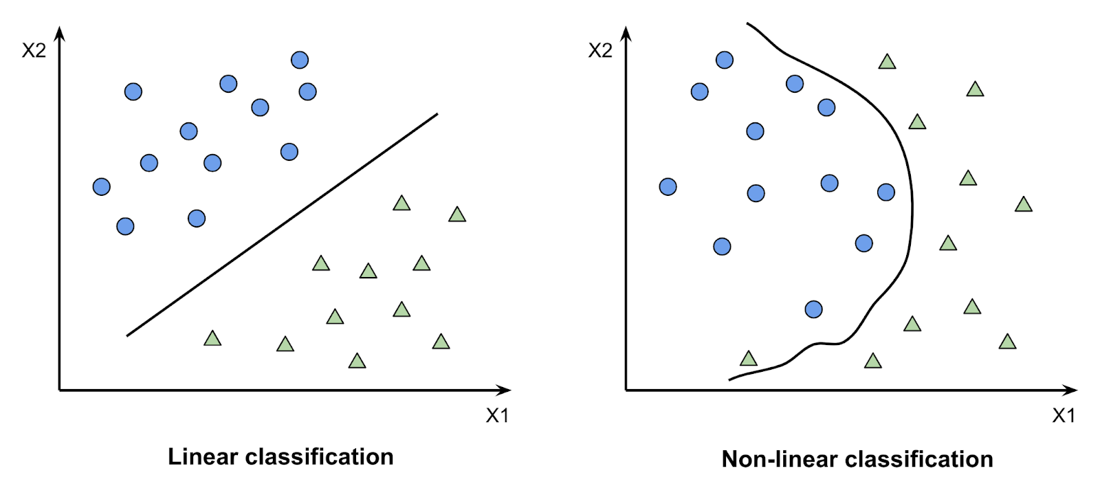
SVM is an algorithm that is used to solve classification problems. Although not so common, it can also be used to solve regression and outlier problems. In the SVM algorithm, a kernel function is applied for accurate prediction. A kernel function is a special mathematical function that takes data as input and converts it into a required form. This transformation of the data is based on something called a kernel trick, which is what gives the kernel function its name. Using the kernel function, we can transform the data that is not linearly separable (cannot be separated using a straight line) into one that is linearly separable.

For binary classification, when the raw output resulting from the kernel function is >= 0, the algorithm predicts a 1, otherwise, it predicts 0. However, the cost calculation for this is that if the actual value is 1 and the model predicts >= 1, there is no cost at all. But if the predicted value < 1, the cost increases as the value of the raw output from the model decreases. You may be wondering, if the raw output >= 0 is predicted as 1, why does the cost start to increase from 1 and below, instead of from 0? This is because SVM punishes both incorrect predictions and predictions that are close to the decision boundary. With the actual value being 1, the decision boundary are values between 0 and 1 inclusively. The values that fall right on the margin and in this decision boundary are called support vectors.

In SVM, there are four types of kernel functions:

• Linear kernel
• Polynomial kernel
• Radial basis kernel
• Sigmoid kernel

Objective functions of SVM:

• Hinge loss: The loss function measures the error between a predicted and actual label. It is a way of measuring how well a model performs from training data to unseen data. Hinge loss is a loss function used for SVM.
• SVM cost function: the cost function is an objective function that is summed up over multiple data points. For example, it could be the sum of the loss function over the training set.

Why SVM?

The last section extensively explained the SVM algorithm. However, you may still be wondering why you should employ this algorithm for your next multi-classification problem. Here are a few advantages of using SVM to train your model:

• The number of observations required to train an SVM isn’t high, so you need less training data.
• SVM can handle both linear and non-linear decision boundaries. It is also parametric and gives high accuracy, most times.
• It performs well in high-dimensional data. That is, data where the number of features is close to or more than the number of observations in the dataset.

Assumptions for using SVMs

Some assumptions of SVMs that help in a good performance are:

1. The dataset is independent and identically distributed across classes. This means that there is a clear distinction between data points in each class.
2. Data does not have a lot of noise and outliers.

LIBSVM

One popular SVM package is the LIBSVM package. LIBSVM is an integrated package for Support Vector Machine classification, regression, and multi-class classification. In the notebook below, I will use LIBSVM to build a classifier model for the UCI wine dataset. LIBSVM is built on C++ and Java sources but has interfaces in many other languages like Python, MATLAB, R, Haskell, Perl, PHP, etc.

I will use the Python interface in a Jupyter notebook; importing it via cloning it from GitHub and building the package.

Parameters of LIBSVM

1. Type of SVM: LIBSVM supports Support Vector Classification (SVC) problems, binary and multi-class, e.g C-SVC and nu-SVC, Support Vector Regression (SVR) problems, e.g epsilon-SVR and nu-SVR, and One-class SVM.
   • C, representing cost, is a regularization parameter. It is set for C-SVC, epsilon-SVR, and nu-SVR SVMs. It should always be positive and the default value is 1.0
   • Nu is a parameter used to control the number of support vectors. It does this by setting the upper bound on the fraction of margin errors and a lower bound on the fraction of support vectors. The default value is 0.5 and it should always be in the interval [0, 1]
2. Kernel type: The different types of kernels that can be applied via LIBSVM are linear, polynomial, Radial Basis Function (RBF), and sigmoid kernels. In general, the RBF kernel is a reasonable first choice when using SVM. This is because it is a non-linear kernel so it can handle situations where the relationship between class labels and attributes is not linear.
3. Other hyperparameters: Some of these include gamma, degree, and coefficients for the kernel function, etc. A full list of these can be found in the official documentation.

How to classify data into multiple classes using LIBSVM in eight steps:

1. Obtain data and carry out EDA to understand the dataset: Read the dataset and carry out exploratory data analysis to understand the data in the dataset. For this demo, I will be using the UCI wine dataset. It is a multiclass classification dataset with 178 records and 13 features. There are three classes of wine as labels in the dataset. The aim is to use chemical analysis to determine the origin of wines. Link to notebook cells:

# Data from http://archive.ics.uci.edu/ml/datasets/Wine
!git clone https://gist.github.com/tijptjik/9408623

# Read in as a dataframe for EDA
wine_df = pd.read_csv('9408623/wine.csv')
print(wine_df.head())
print(wine_df.describe())
print(wine_df.columns)
print(wine_df.dtypes)

# Read in data as an array to begin analysis. Drop header row as it is # not needed for svm classification.
wine_data = np.genfromtxt('9408623/wine.csv', delimiter=',')
wine_data = wine_data[1:] 

print(wine_data[0])

2. Preprocess data and prepare in LIBSVM format:
   1. SVM data only takes in numerical data. If you have categorical data, like text, dates, or time, you have to convert these to numeric values.
   2. Also, SVM does not perform well with wide-ranged data. For a good-performing model, you have to scale your data. The good thing about LIBSVM is that there is an executable to scale the data. I will talk more about this in step 4.
   3. While parsing the data, please make sure there is no trailing new line (‘\n’) as this could cause an error when scaling and training.
   4. Finally, the LIBSVM format is label index:feature…
      label 1:feature1_value 2:feature2_value 3:feature3_value
      and so on, for each row in the dataset. An example is:
      2 1: 0.22 2: 0.45 …
      where 2 is the label, and 1, 2, …, ... depict the index of the features with their corresponding values.
   5. The datatype of the labels and indices are integers, while the feature values could be integers or floats.
   6. In your dataset, there should be no colon (:) even after the hashtag as a comment. This is because the model takes a colon as a feature, hence, it will throw an error since it is not. The only colons allowed are between an index and the feature value for that index.

# Adding count, beginning from 1, to features for each row

with_features_index = []
data_with_features_index = []

for j in range(len(wine_data)):
    each_row = wine_data[j,0:]

    with_features_index.append(each_row[0])

    for l in range(1,14):
        with_features_index.append(str(l)+ ":" + str(each_row[l]))

    data_with_features_index.append(with_features_index)  
    with_features_index = []

3. Split data into train and test datasets: Now that we have read our data, explored it to understand it better, preprocessed, and reformatted it to the LIBSVM format, the next step is to split the dataset into train and test datasets. Because I will carry out cross-validation, I opted for a test size of 0.33, to allow for a larger training dataset.

# Split into train and test datasets
train_data, test_data = train_test_split(data_with_features_index, test_size=0.33, random_state=42)

# Convert to Numpy array
train_data = np.asarray(train_data)
test_data = np.asarray(test_data)
    
# Get y_label from test data to compare against model result later
y_label = np.array(test_data[:,0], dtype=np.float32)
y_label

# Save train and test data to files
np.savetxt('wine_svm_train_data', train_data, delimiter=" ", fmt="%s") 
np.savetxt('wine_svm_test_data', test_data, delimiter=" ", fmt="%s") 

4. Scale data: As mentioned in step 2, you want to scale your data when building SVM model. This is because SVM is an algorithm based on measuring how far apart data points are, and classifying them. Another algorithm like this is the k-nearest neighbors (KNN). Scaling also helps to avoid attributes in greater numeric ranges dominating those in smaller numeric ranges. When scaling your data, you should use the same scale range text for the train and test datasets. So when you scale the train dataset, you save the range text for the train data, then load the range text and use that to scale the test data. This is so that both datasets are scaled in exactly the same way. I scaled the data to [-1,1]. These values are passed as -l and -u arguments in the svm-scale command, l meaning lower bound and u being the upper bound. Using an RBF kernel, which is what we are using, scaling the data between [0,1] and [-1,1] performs the same, so you can use either that you prefer. However, computation time might differ even though performance is the same so this is something you can experiment with. If you have many zero entries, scaling [0,1], as opposed to [-1,1] maintains the sparse nature of the data and may reduce computation time.

5. Carry out cross-validation: I used the LIBSVM grid.py script to handle cross-validation. Cross-validation is the process of subsetting the training data into k-folds of validation datasets to find the right hyperparameters for the model. I set the number of folds for cross-validation to 5 folds. This is set via the -v argument in the grid.py command. Grid.py also has the functionality to use gnuplot to plot a contour of accuracy for each set of hyperparameters from cross-validation. However, I did not use this due to installation and access roadblocks with gnuplot on different systems. This is to maintain the reproducibility of the notebook. But, if you will like to try this out regardless, you can check out this repository on how to get gnuplot in a notebook, then replace the “null” value in the grid.py command with the path to your gnuplot executable. The hyperparameters I tuned are the C and g parameters:

   • C: (cost) - C is the regularization parameter to prevent overfitting and control boundary error in a C-SVC. The default value is 1. A lower value of C gives a simpler decision function, at the cost of training accuracy. This allows more values in the decision boundary; as opposed to a higher C value that gives a slimmer decision boundary.
   • g: (gamma) - set gamma in kernel function (default 1/num_features). A lower value of g gives a constrained model that cannot fully capture the entire complexity of the dataset. It could easily lead to higher variance and overfitting, despite C being a regularization parameter to manage this.

6. Train the model: After cross-validation, I train the model using the best hyperparameters gotten. This model is saved to a model file which is loaded to make predictions on the test data (unseen data). This is done by calling the svm-train executable from the LIBSVM package. I coupled the scaling, training, and testing process into a function. So you carry out these steps, by calling the svm_model function with the filenames of the train and test datasets from Step 3 as parameters.

# Function to scale, train, and test model

def svm_model(train_pathname, test_pathname):

  # Validate that train and test files exist
  assert os.path.exists(train_pathname),"training file not found"
  file_name = os.path.split(train_pathname)[1]

  # Create files to store scaled train data, range metadata for scaled data, and trained model
  scaled_file = file_name + ".scale"
  model_file = file_name + ".model"
  range_file = file_name + ".range" # store scale range for train data to be used to scale test data

  file_name = os.path.split(test_pathname)[1]
  assert os.path.exists(test_pathname),"testing file not found"

  # Create file for scaled test data and predicted output
  scaled_test_file = file_name + ".scale"
  predict_test_file = file_name + ".predict"

  # Scaling by range [-1, 1]
  cmd = '{0} -l {4} -u {5} -s "{1}" "{2}" > "{3}"'.format(svmscale_exe, range_file, train_pathname, scaled_file, -1, 1)
  print('Scaling train data')
  Popen(cmd, shell = True, stdout = PIPE).communicate()

  # Tuning c and g hyperparameters using a 5-fold grid search
  cmd = '{0} -v {4} -svmtrain "{1}" -gnuplot "{2}" "{3}"'.format(grid_py, svmtrain_exe, "null", scaled_file, 5)
  print('Cross validation')
  f = Popen(cmd, shell = True, stdout = PIPE).stdout

  line = ''
  while True:
      last_line = line
      line = f.readline()
      if not line: break
  c,g,rate = map(float,last_line.split())

  print('Best c={0}, g={1} CV rate={2}'.format(c,g,rate))

  cmd = '{0} -c {1} -g {2} "{3}" "{4}"'.format(svmtrain_exe,c,g,scaled_file,model_file)
  print('Training model')
  Popen(cmd, shell = True, stdout = PIPE).communicate()

  print('Output model: {0}'.format(model_file))

  cmd = '{0} -l {4} -u {5} -r "{1}" "{2}" > "{3}"'.format(svmscale_exe, range_file, test_pathname, scaled_test_file, -1, 1)
  print('Scaling test data')
  Popen(cmd, shell = True, stdout = PIPE).communicate()

  cmd = '{0} "{1}" "{2}" "{3}"'.format(svmpredict_exe, scaled_test_file, model_file, predict_test_file)
  print('Testing model\n')
  f = Popen(cmd, shell = True, stdout = PIPE).stdout
  result = (str(f.readline()).replace("\\n'", '')).replace("b'", '')
  print("{} \n".format(result))

  print('Output prediction: {0}'.format(predict_test_file))

7. Test model on test data: To test the model, the svm-predict executable command is called with the saved model, best hyper parameter values for c and g, as well as, the scaled test data. The output of this is stored in predict file and it is an array of the predicted classes for each row in the test dataset. For this problem, I will be using accuracy as a measure of performance. Accuracy is a good measure of performance for this demo because of the nature of the problem, classification of wine origins, and the count of the different classes not being imbalanced. However, if your classes are imbalanced, accuracy may not be the best metric. Also, for some problems, precision or recall or novelty, or some other metric may give better insights into the model performance for that problem, so don’t feel obligated to always use accuracy. The test accuracy of the model was 98.3051% with 58 out of 59 data points in our dataset being correctly classified. This was such an excellent performance, and I decided not to do further tweaking to the model or hyperparameters.

svm_model(wine_svm_data_train_file, wine_svm_data_test_file)

8. Evaluate the performance of the model: To evaluate the model, I tested the model trained with the best hyperparameters on unseen (test) data and used scikit-learn to plot the confusion matrix. From the confusion matrix, the one wrong classification was in class 2.

def evaluate_model(y_label, predict_test_file):


  # Creating the y_label for the confusion matrix
  f=open(predict_test_file,'r')
  y_pred = np.genfromtxt(f,dtype = 'float')

  # Confusion matrix
  cf_matrix = confusion_matrix(y_label, y_pred)

  # Plot heatmap
  ax = sns.heatmap(cf_matrix/np.sum(cf_matrix), annot=True, 
          fmt='.2%', cmap='Blues')

  # Format plot
  ax.set_title('Seaborn Confusion Matrix with wine class labels\n\n');
  ax.set_xlabel('\nPredicted action')
  ax.set_ylabel('Actual action ');

  # Ticket labels - List must be in alphabetical order
  ax.xaxis.set_ticklabels(['1', '2', '3'])
  ax.yaxis.set_ticklabels(['1', '2', '3'])

  # Display the visualization of the Confusion Matrix.
  plt.show()

evaluate_model(y_label, 'wine_svm_test_data.predict')

Limitations

SVM, and particularly LIBSVM, has some limitations as a machine learning algorithm for classification. In this section, I will mention some of them, so that you can be aware and keep these in mind when considering this algorithm for your classification needs.

1. Requires unique format of input data, labeled for each feature.
2. Due to its use in high-dimensional spaces, it is prone to overfitting. You can avoid this by choosing a suitable kernel function and setting the regularization parameters.
3. The cross-validation technique involved is expensive to compute for large datasets.
4. Data has to be scaled and within a close range for the best results.
5. There is no probabilistic explanation for the classification of observations.

Conclusion

We just walked through multi-class classification using LIBSVM. SVM is a great machine learning algorithm for classification because it does not require a very large training dataset, can work with many features, and can handle linear and non-linear boundaries. LIBSVM is a good SVM package, especially, for beginners because most of the tweaking is abstracted for you, yet still yields very high performance. Hopefully, from this article, you have been able to get your hands dirty with classifying data into multiple classes using SVM. Please find the full notebook that was used here.

Thank you for reading.

References

1. Chih-Chung Chang and Chih-Jen Lin, LIBSVM : a library for support vector machines. ACM Transactions on Intelligent Systems and Technology, 2:27:1--27:27, 2011. Software available at http://www.csie.ntu.edu.tw/~cjlin/libsvm
2. https://www.csie.ntu.edu.tw/~cjlin/papers/guide/guide.pdf
3. https://www.csie.ntu.edu.tw/~cjlin/libsvm/faq.html
4. Dua, D. and Graff, C. (2019). UCI Machine Learning Repository [http://archive.ics.uci.edu/ml]. Irvine, CA: University of California, School of Information and Computer Science.
5. https://www.csie.ntu.edu.tw/~cjlin/papers/libsvm.pdf