Step-by-step instructions for training YOLOv7 on a Custom Dataset

Follow this guide to get step-by-step instructions for running YOLOv7 model training within a Gradient Notebook on a custom dataset. This tutorial is based on our popular guide for running YOLOv5 custom training with Gradient, and features updates to work with YOLOv7.

We will first set up the Python code to run in a notebook. Next, we will download the custom dataset, and convert the annotations to the Yolov7 format. There are provided helper functions to make it easy to test that the annotations match the images. We will then partition the dataset into training and validation sets. For training, we will then establish several training options, and set up our data  and hyper parameter configuration files. We will then walk through how we can modify the network architecture as needed for our custom data. Once set up is complete, we will show how to train the model for 100 epochs, and then use it to generate predictions on our validation set. We will then use the results to compute the mAP on the test data, so that we may assess the quality of the final model.

Set up the code

We begin by cloning the YOLOv7 repository and setting up the dependencies required to run YOLOv7. If you are using the Run on Gradient link from above, this step will be done for you. You can also make the YOLOv7 repo your workspace directory using the advanced options toggle in the Notebook creation page.

Next, we will install the required packages. In a terminal (or using cell magic), type:

pip install -r requirements.txt

Note: The step above is not needed if you are working in a Gradient Notebook - these packages have already been installed.

With the dependencies installed, we will then import the required modules to conclude setting up the Notebook.

import torch
from IPython.display import Image  # for displaying images
import os 
import random
import shutil
from sklearn.model_selection import train_test_split
import xml.etree.ElementTree as ET
from xml.dom import minidom
from tqdm import tqdm
from PIL import Image, ImageDraw
import numpy as np
import matplotlib.pyplot as plt

random.seed(108)

Download the Data

For this tutorial, we are going to use an object detection dataset of road signs from MakeML. We can source this data from Kaggle in just a few steps.

To do this, first we will create a directory called Road_Sign_Dataset to keep our dataset. The directory needs to be in the same folder as the YOLOv7 repository folder we just cloned/that is our workspace directory in the Notebook.

mkdir Road_Sign_Dataset
cd Road_Sign_Dataset

To download the dataset from Kaggle for a Gradient Notebook, first get a Kaggle account. Next, create an API token by going to your Account settings, and save kaggle.json to your local machine. Upload kaggle.json to the Gradient Notebook. Finally, run the code cell below to download the zip file.

pip install kaggle
mkdir ~/.kaggle
mv kaggle.json ~/.kaggle
kaggle datasets download andrewmvd/road-sign-detection

Unzip the dataset.

unzip road-sign-detection.zip

Delete the unneeded files.

rm -r road-sign-detection.zip

Exploring the Dataset

The dataset we are using for this example is a relatively small one, containing only 877 images in total. The recommended usual value is above 3000 images per class. We could apply all the same techniques used for this dataset with a larger dataset (like the LISA Dataset) to fully realize the capabilities of YOLO, but we are going to use a small dataset in this tutorial to facilitate quick prototyping. Typical training takes less than half an hour and this would allow you to quickly iterate with experiments involving different hyperparamters.

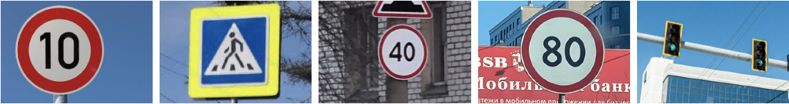
The dataset contains road signs belonging to 4 classes:

1. Traffic Lights
2. Stop signs
3. Speed Limit signs
4. Crosswalk signs

Convert the Annotations into the YOLO v5 Format

Now that we have our dataset, we need to convert the annotations into the format expected by YOLOv7. YOLOv7 expects data to be organized in a specific way, otherwise it is unable to parse through the directories. Reordering our data will ensure that we have no problems initiating training.

The annotations for the Road Sign Detection dataset all follow the PASCAL VOC XML format. This a very popular format, since it is simplistic to store multiple types of data in a single table structure. Since this a popular format, there are a number of simple to use online conversion tools to reformat XML data. Nevertheless, we have provided code to show how to convert other popular formats as well (for which you may not find popular tools).

The PASCAL VOC format stores its annotation in XML files where each of its various attributes are described by tags. Let us look at an example annotation file.

# Assuming you're in the data folder
cat annotations/road4.xml

The output looks like the following.

<annotation>
    <folder>images</folder>
    <filename>road4.png</filename>
    <size>
        <width>267</width>
        <height>400</height>
        <depth>3</depth>
    </size>
    <segmented>0</segmented>
    <object>
        <name>trafficlight</name>
        <pose>Unspecified</pose>
        <truncated>0</truncated>
        <occluded>0</occluded>
        <difficult>0</difficult>
        <bndbox>
            <xmin>20</xmin>
            <ymin>109</ymin>
            <xmax>81</xmax>
            <ymax>237</ymax>
        </bndbox>
    </object>
    <object>
        <name>trafficlight</name>
        <pose>Unspecified</pose>
        <truncated>0</truncated>
        <occluded>0</occluded>
        <difficult>0</difficult>
        <bndbox>
            <xmin>116</xmin>
            <ymin>162</ymin>
            <xmax>163</xmax>
            <ymax>272</ymax>
        </bndbox>
    </object>
    <object>
        <name>trafficlight</name>
        <pose>Unspecified</pose>
        <truncated>0</truncated>
        <occluded>0</occluded>
        <difficult>0</difficult>
        <bndbox>
            <xmin>189</xmin>
            <ymin>189</ymin>
            <xmax>233</xmax>
            <ymax>295</ymax>
        </bndbox>
    </object>
</annotation>

The above annotation file describes a file named road4.jpg. We can see that it has dimensions of 267 x 400 x 3. It also has 3 object tags, which each represent 3 corresponding bounding boxes. The class is specified by the name tag, and the positioning of the bounding box coordinates are represented by the bndbox tag. A bounding box is described by the coordinates of its top-left (x_min, y_min) corner and its bottom-right (xmax, ymax) corner.

The YOLOv7 Annotation Format

Let's look more closely at the annotation files. YOLOv7 expects annotations for each image in form of a .txt file where each line of the text file describes a bounding box. Consider the following image.

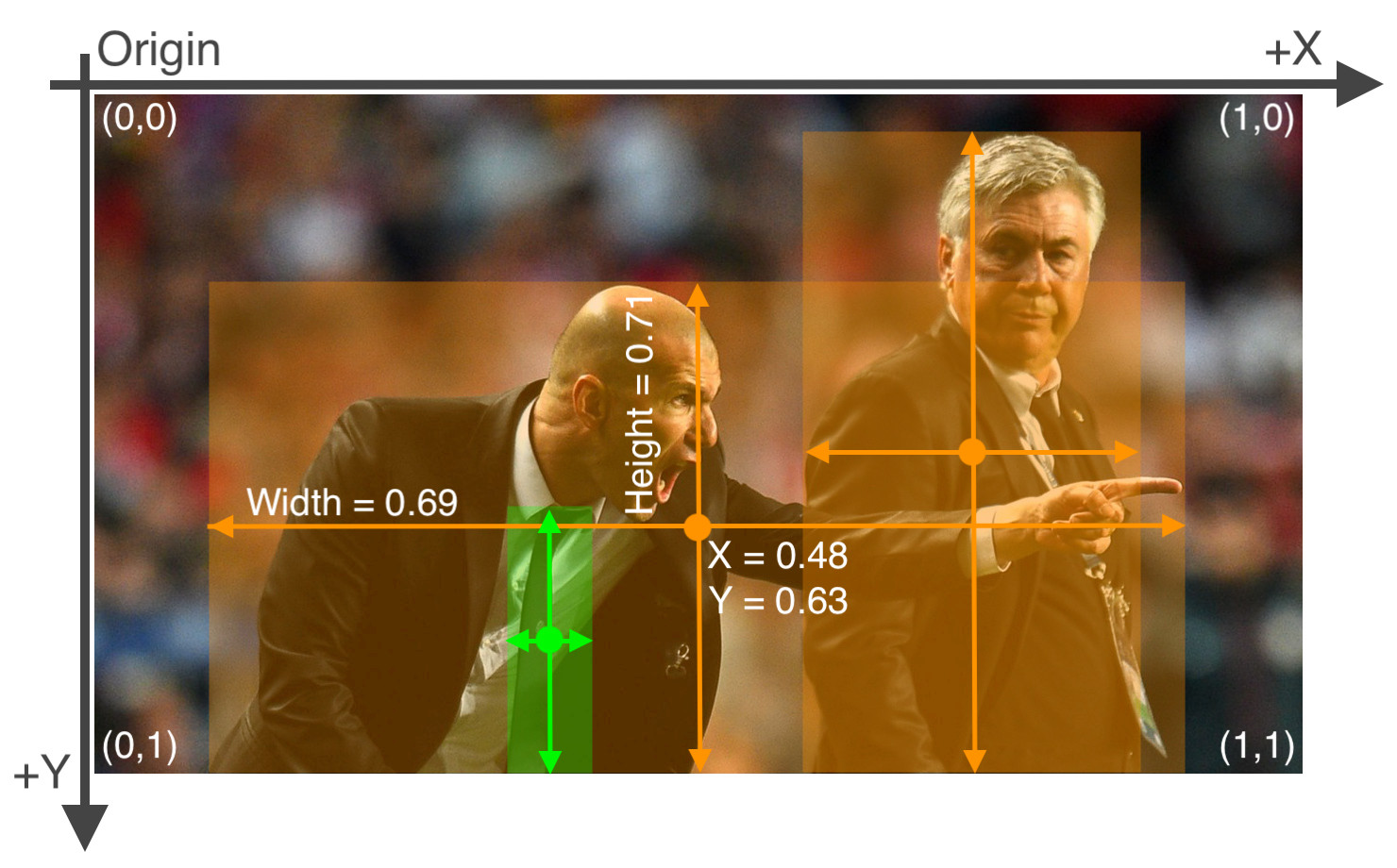
The annotation file for the image contains the coordinates for each of the bounding boxes shown above. The format of these labels will look like the following:

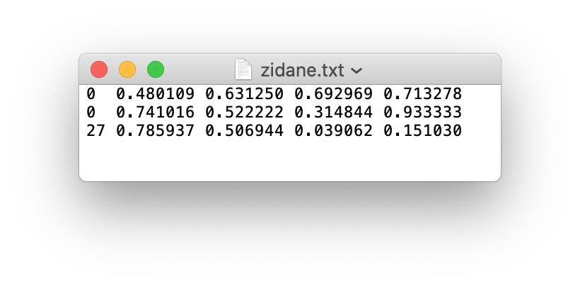
As we can see, there are 3 objects in total (2 persons and one tie). Each line represents one of these objects. The specification for each line is as follows.

• One row per object
• The columns are class, x_center, y_center, width, and height format.
• These box coordinates must be normalized to the dimensions of the image (i.e. have values between 0 and 1)
• Class numbers are zero-indexed (start from 0).

We will next write a function that will take the annotations in VOC format and convert them to a format where information about the bounding boxes is stored in a dictionary.

# Function to get the data from XML Annotation
def extract_info_from_xml(xml_file):
    root = ET.parse(xml_file).getroot()
    
    # Initialise the info dict 
    info_dict = {}
    info_dict['bboxes'] = []

    # Parse the XML Tree
    for elem in root:
        # Get the file name 
        if elem.tag == "filename":
            info_dict['filename'] = elem.text
            
        # Get the image size
        elif elem.tag == "size":
            image_size = []
            for subelem in elem:
                image_size.append(int(subelem.text))
            
            info_dict['image_size'] = tuple(image_size)
        
        # Get details of the bounding box 
        elif elem.tag == "object":
            bbox = {}
            for subelem in elem:
                if subelem.tag == "name":
                    bbox["class"] = subelem.text
                    
                elif subelem.tag == "bndbox":
                    for subsubelem in subelem:
                        bbox[subsubelem.tag] = int(subsubelem.text)            
            info_dict['bboxes'].append(bbox)
    
    return info_dict

Let us try this function on a sample annotation file.

print(extract_info_from_xml('annotations/road4.xml'))

This outputs:

{'bboxes': [{'class': 'trafficlight', 'xmin': 20, 'ymin': 109, 'xmax': 81, 'ymax': 237}, {'class': 'trafficlight', 'xmin': 116, 'ymin': 162, 'xmax': 163, 'ymax': 272}, {'class': 'trafficlight', 'xmin': 189, 'ymin': 189, 'xmax': 233, 'ymax': 295}], 'filename': 'road4.png', 'image_size': (267, 400, 3)}

This effectively extracts the information needed to use with YOLOv7.

Next, we will create a function to convert this information, now contained in info_dict, to YOLOv7 style annotations and write them to txt files. If our annotations are different than PASCAL VOC ones, we can write a new function to convert them to the info_dict format, and use the same function below to convert them to YOLOv7 style annotations. As long as the info-dict format is conserved, this code should work.

# Dictionary that maps class names to IDs
class_name_to_id_mapping = {"trafficlight": 0,
                           "stop": 1,
                           "speedlimit": 2,
                           "crosswalk": 3}

# Convert the info dict to the required yolo format and write it to disk
def convert_to_yolov5(info_dict):
    print_buffer = []
    
    # For each bounding box
    for b in info_dict["bboxes"]:
        try:
            class_id = class_name_to_id_mapping[b["class"]]
        except KeyError:
            print("Invalid Class. Must be one from ", class_name_to_id_mapping.keys())
        
        # Transform the bbox co-ordinates as per the format required by YOLO v5
        b_center_x = (b["xmin"] + b["xmax"]) / 2 
        b_center_y = (b["ymin"] + b["ymax"]) / 2
        b_width    = (b["xmax"] - b["xmin"])
        b_height   = (b["ymax"] - b["ymin"])
        
        # Normalise the co-ordinates by the dimensions of the image
        image_w, image_h, image_c = info_dict["image_size"]  
        b_center_x /= image_w 
        b_center_y /= image_h 
        b_width    /= image_w 
        b_height   /= image_h 
        
        #Write the bbox details to the file 
        print_buffer.append("{} {:.3f} {:.3f} {:.3f} {:.3f}".format(class_id, b_center_x, b_center_y, b_width, b_height))
        
    # Name of the file which we have to save 
    save_file_name = os.path.join("annotations", info_dict["filename"].replace("png", "txt"))
    
    # Save the annotation to disk
    print("\n".join(print_buffer), file= open(save_file_name, "w"))

Next, we use this function with each xml file to convert all of the xml annotations into YOLO style txt ones.

# Get the annotations
annotations = [os.path.join('annotations', x) for x in os.listdir('annotations') if x[-3:] == "xml"]
annotations.sort()

# Convert and save the annotations
for ann in tqdm(annotations):
    info_dict = extract_info_from_xml(ann)
    convert_to_yolov5(info_dict)
annotations = [os.path.join('annotations', x) for x in os.listdir('annotations') if x[-3:] == "txt"]

Testing the annotations

Let us now test some of these transformed annotations, and make sure they are in the correct format. The code below will randomly load one of the annotations, and use it to plot boxes with the transformed annotations. We can then visually inspect it to see whether our code has worked as intended.

Our suggestion is to run the next cell multiple times. Every time, a random annotation is sampled, and we can see that the data was correctly ordered.

random.seed(0)

class_id_to_name_mapping = dict(zip(class_name_to_id_mapping.values(), class_name_to_id_mapping.keys()))

def plot_bounding_box(image, annotation_list):
    annotations = np.array(annotation_list)
    w, h = image.size
    
    plotted_image = ImageDraw.Draw(image)

    transformed_annotations = np.copy(annotations)
    transformed_annotations[:,[1,3]] = annotations[:,[1,3]] * w
    transformed_annotations[:,[2,4]] = annotations[:,[2,4]] * h 
    
    transformed_annotations[:,1] = transformed_annotations[:,1] - (transformed_annotations[:,3] / 2)
    transformed_annotations[:,2] = transformed_annotations[:,2] - (transformed_annotations[:,4] / 2)
    transformed_annotations[:,3] = transformed_annotations[:,1] + transformed_annotations[:,3]
    transformed_annotations[:,4] = transformed_annotations[:,2] + transformed_annotations[:,4]
    
    for ann in transformed_annotations:
        obj_cls, x0, y0, x1, y1 = ann
        plotted_image.rectangle(((x0,y0), (x1,y1)))
        
        plotted_image.text((x0, y0 - 10), class_id_to_name_mapping[(int(obj_cls))])
    
    plt.imshow(np.array(image))
    plt.show()

# Get any random annotation file 
annotation_file = random.choice(annotations)
with open(annotation_file, "r") as file:
    annotation_list = file.read().split("\n")[:-1]
    annotation_list = [x.split(" ") for x in annotation_list]
    annotation_list = [[float(y) for y in x ] for x in annotation_list]

#Get the corresponding image file
image_file = annotation_file.replace("annotations", "images").replace("txt", "png")
assert os.path.exists(image_file)

#Load the image
image = Image.open(image_file)

#Plot the Bounding Box
plot_bounding_box(image, annotation_list)

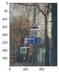
Great, we are able to recover the correct annotation from the YOLOv7 format. This means we have implemented the conversion function properly.

Partition the Dataset

Next, we need to partition the dataset into train, validation, and test sets. These will contain 80%, 10%, and 10% of the data, respectively. These values can be edited to change the split percentages, as needed.

# Read images and annotations
images = [os.path.join('images', x) for x in os.listdir('images')]
annotations = [os.path.join('annotations', x) for x in os.listdir('annotations') if x[-3:] == "txt"]

images.sort()
annotations.sort()

# Split the dataset into train-valid-test splits 
train_images, val_images, train_annotations, val_annotations = train_test_split(images, annotations, test_size = 0.2, random_state = 1)
val_images, test_images, val_annotations, test_annotations = train_test_split(val_images, val_annotations, test_size = 0.5, random_state = 1)

We will then create the folders to hold our newly split data.

!mkdir images/train images/val images/test labels/train labels/val labels/test

Finally, we finish setting up the data by moving the files to their respective folders.

#Utility function to move images 
def move_files_to_folder(list_of_files, destination_folder):
    for f in list_of_files:
        try:
            shutil.move(f, destination_folder)
        except:
            print(f)
            assert False

# Move the splits into their folders
move_files_to_folder(train_images, 'images/train')
move_files_to_folder(val_images, 'images/val/')
move_files_to_folder(test_images, 'images/test/')
move_files_to_folder(train_annotations, 'annotations/train/')
move_files_to_folder(val_annotations, 'annotations/val/')
move_files_to_folder(test_annotations, 'annotations/test/')
!mv annotations labels
%cd ../

Training Options

Now, it's time to set up our options for training the network. We will make use of various flags to do so, including:

• img-size: This parameter corresponds to the size of the image in pixels. For YOLOv7, The image must be square one. To make it so, the original image is resized while maintaining the aspect ratio. The longer side of the image is resized to this number. The shorter side is padded with grey color.

• batch: The batch size corresponds to the number of image-caption pairs being propagated through the network at any given time during training
• epochs: Number of epochs to train for. This value corresponds to the total number of passes the model training will take across the entire dataset
• data: The Data YAML file contains information about the dataset to help direct YOLO. Information inside includes path to the images, the number of class labels, and the names of the class labels
• workers: Indicates the number of CPU workers being allocated for training
• cfg: The configuration file for the model architecture. There are possible choices are yolov7-e6e.yaml, yolov7-d6.yaml, yolov7-e6.yaml, yolov7-w6.yaml, yolov7x.yaml, yolov7.yaml, and yolov7-tiny.yaml. The size and complexity of these models increases in the descending order, and we can use these to best select the model which suits the complexity of our object detection task. In cases where we want to work with a custom architecture, we will have to define a YAML file in the cfg folder specifying the network architecture
• weights: Pretrained model weights we will want to re-start training from. If we want to train from scratch, we can just use --weights ' '
• name: The path for various outputs about training such as train logs. The outputted training weights, logs, and samples of batched images are stored in a folder corresponding to runs/train/<name>.
• hyp: YAML file that describes hyperparameter choices for the model training. For examples of how to define custom hyperparameters, see data/hyp.scratch.yaml. If unspecified, the hyperparameters in data/hyp.scratch.yaml is used.

Data Config File

Details for the dataset you want to train your model on are defined by the data config YAML file. The following parameters have to be defined in a data config file:

1. train, test, and val: Paths for train, test, and validation images
2. nc: Number of classes in the dataset
3. names: Names of the class labels in the dataset. The index of the classes in this list can be used as an identifier for the class names in the code.

We can create a new file called road_sign_data.yaml and place it in the data folder. Then populate it with the following.

train: Road_Sign_Dataset/images/train/ 
val:  Road_Sign_Dataset/images/val/
test: Road_Sign_Dataset/images/test/

# number of classes
nc: 4

# class names
names: ["trafficlight","stop", "speedlimit","crosswalk"]

YOLOv7 expects to find the corresponding training labels for the images in the folder whose name is derived by replacing images with labels in the path to dataset images. For example, in the example above, YOLO v5 will look for train labels in Road_Sign_Dataset/labels/train/.

Alternatively, we can skip this step by simply downloading the file to our working directory's data folder.

!wget -P data/ https://gist.githubusercontent.com/ayooshkathuria/bcf7e3c929cbad445439c506dba6198d/raw/f437350c0c17c4eaa1e8657a5cb836e65d8aa08a/road_sign_data.yaml

Hyperparameter Config File

The hyperparameter configuration file helps us define the hyperparameters for our neural network. This gives us a lot of control over the behavior of our model training, and more advanced users should consider modifying certain values like the learning rate if training is not proceeding as desired. It may be able to improve the final outcomes.

We are going to use the default configuration spec, data/hyp.scratch.yaml. This is what it looks like:

# Hyperparameters for COCO training from scratch
# python train.py --batch 40 --cfg yolov5m.yaml --weights '' --data coco.yaml --img 640 --epochs 300
# See tutorials for hyperparameter evolution https://github.com/ultralytics/yolov5#tutorials


lr0: 0.01  # initial learning rate (SGD=1E-2, Adam=1E-3)
lrf: 0.2  # final OneCycleLR learning rate (lr0 * lrf)
momentum: 0.937  # SGD momentum/Adam beta1
weight_decay: 0.0005  # optimizer weight decay 5e-4
warmup_epochs: 3.0  # warmup epochs (fractions ok)
warmup_momentum: 0.8  # warmup initial momentum
warmup_bias_lr: 0.1  # warmup initial bias lr
box: 0.05  # box loss gain
cls: 0.5  # cls loss gain
cls_pw: 1.0  # cls BCELoss positive_weight
obj: 1.0  # obj loss gain (scale with pixels)
obj_pw: 1.0  # obj BCELoss positive_weight
iou_t: 0.20  # IoU training threshold
anchor_t: 4.0  # anchor-multiple threshold
# anchors: 3  # anchors per output layer (0 to ignore)
fl_gamma: 0.0  # focal loss gamma (efficientDet default gamma=1.5)
hsv_h: 0.015  # image HSV-Hue augmentation (fraction)
hsv_s: 0.7  # image HSV-Saturation augmentation (fraction)
hsv_v: 0.4  # image HSV-Value augmentation (fraction)
degrees: 0.0  # image rotation (+/- deg)
translate: 0.1  # image translation (+/- fraction)
scale: 0.5  # image scale (+/- gain)
shear: 0.0  # image shear (+/- deg)
perspective: 0.0  # image perspective (+/- fraction), range 0-0.001
flipud: 0.0  # image flip up-down (probability)
fliplr: 0.5  # image flip left-right (probability)
mosaic: 1.0  # image mosaic (probability)
mixup: 0.0  # image mixup (probability)

You can edit this file as needed, save it, and specify it as an argument to the train script with the hyp option.

Custom Network Architecture

YOLOv7 also allows us to define our own custom architecture and anchors if one of the pre-defined networks doesn't quite fit our task. To take advantage of this, we would have to define a custom weights configuration file or just use one of their premade specs. For this demo, we don't need to make any alterations, and are just going to use the yolov7.yaml. This is what it looks like:

# parameters
nc: 80  # number of classes
depth_multiple: 1.0  # model depth multiple
width_multiple: 1.0  # layer channel multiple

# anchors
anchors:
  - [12,16, 19,36, 40,28]  # P3/8
  - [36,75, 76,55, 72,146]  # P4/16
  - [142,110, 192,243, 459,401]  # P5/32

# yolov7 backbone
backbone:
  # [from, number, module, args]
  [[-1, 1, Conv, [32, 3, 1]],  # 0
  
   [-1, 1, Conv, [64, 3, 2]],  # 1-P1/2      
   [-1, 1, Conv, [64, 3, 1]],
   
   [-1, 1, Conv, [128, 3, 2]],  # 3-P2/4  
   [-1, 1, Conv, [64, 1, 1]],
   [-2, 1, Conv, [64, 1, 1]],
   [-1, 1, Conv, [64, 3, 1]],
   [-1, 1, Conv, [64, 3, 1]],
   [-1, 1, Conv, [64, 3, 1]],
   [-1, 1, Conv, [64, 3, 1]],
   [[-1, -3, -5, -6], 1, Concat, [1]],
   [-1, 1, Conv, [256, 1, 1]],  # 11
         
   [-1, 1, MP, []],
   [-1, 1, Conv, [128, 1, 1]],
   [-3, 1, Conv, [128, 1, 1]],
   [-1, 1, Conv, [128, 3, 2]],
   [[-1, -3], 1, Concat, [1]],  # 16-P3/8  
   [-1, 1, Conv, [128, 1, 1]],
   [-2, 1, Conv, [128, 1, 1]],
   [-1, 1, Conv, [128, 3, 1]],
   [-1, 1, Conv, [128, 3, 1]],
   [-1, 1, Conv, [128, 3, 1]],
   [-1, 1, Conv, [128, 3, 1]],
   [[-1, -3, -5, -6], 1, Concat, [1]],
   [-1, 1, Conv, [512, 1, 1]],  # 24
         
   [-1, 1, MP, []],
   [-1, 1, Conv, [256, 1, 1]],
   [-3, 1, Conv, [256, 1, 1]],
   [-1, 1, Conv, [256, 3, 2]],
   [[-1, -3], 1, Concat, [1]],  # 29-P4/16  
   [-1, 1, Conv, [256, 1, 1]],
   [-2, 1, Conv, [256, 1, 1]],
   [-1, 1, Conv, [256, 3, 1]],
   [-1, 1, Conv, [256, 3, 1]],
   [-1, 1, Conv, [256, 3, 1]],
   [-1, 1, Conv, [256, 3, 1]],
   [[-1, -3, -5, -6], 1, Concat, [1]],
   [-1, 1, Conv, [1024, 1, 1]],  # 37
         
   [-1, 1, MP, []],
   [-1, 1, Conv, [512, 1, 1]],
   [-3, 1, Conv, [512, 1, 1]],
   [-1, 1, Conv, [512, 3, 2]],
   [[-1, -3], 1, Concat, [1]],  # 42-P5/32  
   [-1, 1, Conv, [256, 1, 1]],
   [-2, 1, Conv, [256, 1, 1]],
   [-1, 1, Conv, [256, 3, 1]],
   [-1, 1, Conv, [256, 3, 1]],
   [-1, 1, Conv, [256, 3, 1]],
   [-1, 1, Conv, [256, 3, 1]],
   [[-1, -3, -5, -6], 1, Concat, [1]],
   [-1, 1, Conv, [1024, 1, 1]],  # 50
  ]

# yolov7 head
head:
  [[-1, 1, SPPCSPC, [512]], # 51
  
   [-1, 1, Conv, [256, 1, 1]],
   [-1, 1, nn.Upsample, [None, 2, 'nearest']],
   [37, 1, Conv, [256, 1, 1]], # route backbone P4
   [[-1, -2], 1, Concat, [1]],
   
   [-1, 1, Conv, [256, 1, 1]],
   [-2, 1, Conv, [256, 1, 1]],
   [-1, 1, Conv, [128, 3, 1]],
   [-1, 1, Conv, [128, 3, 1]],
   [-1, 1, Conv, [128, 3, 1]],
   [-1, 1, Conv, [128, 3, 1]],
   [[-1, -2, -3, -4, -5, -6], 1, Concat, [1]],
   [-1, 1, Conv, [256, 1, 1]], # 63
   
   [-1, 1, Conv, [128, 1, 1]],
   [-1, 1, nn.Upsample, [None, 2, 'nearest']],
   [24, 1, Conv, [128, 1, 1]], # route backbone P3
   [[-1, -2], 1, Concat, [1]],
   
   [-1, 1, Conv, [128, 1, 1]],
   [-2, 1, Conv, [128, 1, 1]],
   [-1, 1, Conv, [64, 3, 1]],
   [-1, 1, Conv, [64, 3, 1]],
   [-1, 1, Conv, [64, 3, 1]],
   [-1, 1, Conv, [64, 3, 1]],
   [[-1, -2, -3, -4, -5, -6], 1, Concat, [1]],
   [-1, 1, Conv, [128, 1, 1]], # 75
      
   [-1, 1, MP, []],
   [-1, 1, Conv, [128, 1, 1]],
   [-3, 1, Conv, [128, 1, 1]],
   [-1, 1, Conv, [128, 3, 2]],
   [[-1, -3, 63], 1, Concat, [1]],
   
   [-1, 1, Conv, [256, 1, 1]],
   [-2, 1, Conv, [256, 1, 1]],
   [-1, 1, Conv, [128, 3, 1]],
   [-1, 1, Conv, [128, 3, 1]],
   [-1, 1, Conv, [128, 3, 1]],
   [-1, 1, Conv, [128, 3, 1]],
   [[-1, -2, -3, -4, -5, -6], 1, Concat, [1]],
   [-1, 1, Conv, [256, 1, 1]], # 88
      
   [-1, 1, MP, []],
   [-1, 1, Conv, [256, 1, 1]],
   [-3, 1, Conv, [256, 1, 1]],
   [-1, 1, Conv, [256, 3, 2]],
   [[-1, -3, 51], 1, Concat, [1]],
   
   [-1, 1, Conv, [512, 1, 1]],
   [-2, 1, Conv, [512, 1, 1]],
   [-1, 1, Conv, [256, 3, 1]],
   [-1, 1, Conv, [256, 3, 1]],
   [-1, 1, Conv, [256, 3, 1]],
   [-1, 1, Conv, [256, 3, 1]],
   [[-1, -2, -3, -4, -5, -6], 1, Concat, [1]],
   [-1, 1, Conv, [512, 1, 1]], # 101
   
   [75, 1, RepConv, [256, 3, 1]],
   [88, 1, RepConv, [512, 3, 1]],
   [101, 1, RepConv, [1024, 3, 1]],

   [[102,103,104], 1, IDetect, [nc, anchors]],   # Detect(P3, P4, P5)
  ]

If we wanted to use a custom network, then we could create a new file (like yolov7_training.yaml, and specify it when we are training using the cfg flag.

Training the Model

We have now defined the location of train, val and test, the number of classes (nc), and the names of the classes using our data file, so we are ready to start model training. Since the dataset is relatively small, and we don't have many objects per image, we can start off with the basic version of the available pretrained models, yolosv7.pt, to keep things simple and avoid overfitting. We will be using a batch size of 8, so that this will run on Gradient's Free GPU Notebooks, an image size of 640, and we will train for 100 epochs.

If you are still having issues fitting the model into the memory:

• Use a smaller batch size: try a batch size of 2 or 4 if 8 will not work, but this shouldn't happen on the Free GPU
• Use a smaller network: the yolov7-tiny.pt checkpoint will run at lower cost than the basic yolov7.pt
• Use a smaller image size: the size of the image corresponds directly to expense during training. Reduce the images from 640 to 320 to significantly cut cost at the expense of losing prediction accuracy

Changing any of the above will likely impact performance. The compromise is a design decision we have to make depending on our available compute. We might want to go for a bigger GPU instance as well, depending on the situation. For example, a more powerful GPU like the A100-80G would significantly cut training time, but would be pretty overboard for this smaller dataset training task. Check out our breakdown of YOLOv7 benchmarks here.

We will use the name yolo_road_det for our training. Keep in mind if we are to run training again without changing this, the outputs will redirect to yolo_road_det1, and keep adding to that appended last value as you iterate. The tensorboard training logs can be found at runs/train/yolo_road_det/results.txt. You can also take advantage of the YOLOv7 model's integration with Weights & Biases, and connect a wandb account so that the logs are plotted over on your account.

Finally, we have completed set up, and are ready to train our model. Run the training by executing the code cell below:

!python train.py --img-size 640 --cfg cfg/training/yolov7.yaml --hyp data/hyp.scratch.custom.yaml --batch 8 --epochs 100 --data data/road_sign.yaml --weights yolov7_training.pt --workers 24 --name yolo_road_det

Note: This can take up to 5 hours to train on a Free GPU (M4000). If time is a factor, consider upgrading to one of our more powerful machines.

Inference

There are many ways to run inference using the detect.py file, and generate the predicted labels for the classes in the test set images.

When runing the detect.py code, we again have a number of options we will need to set.

• The source flag defines the source of our detector, which will typically be one of: a single image, a folder of images, a video, or a live feed from some video stream or webcam. We want to run it over our test images so we set the source flag to Road_Sign_Dataset/images/test/.
• The weights option defines the path of the model which we want to run our detector with. We will use the best.pt model from our last training run, which is the quantitative 'best' performing model in terms of mAP on the validation set.
• Theconf flag is the thresholding objectness confidence.
• Thename flag defines where the detections are stored. We set this flag to yolo_road_det; therefore, the detections would be stored in runs/detect/yolo_road_det/.

With all options decided, let us run inference with our test dataset, and see, qualitatively, how our model training has done. Run the code in the cell below:

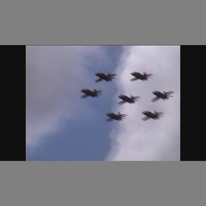
!python detect.py --source Road_Sign_Dataset/images/test/ --weights runs/train/yolo_road_det5/weights/best.pt --conf 0.25 --name yolo_road_det

Once that is completed, we can now randomly plot one of the detections, and see how our training did.

detections_dir = "runs/detect/yolo_road_det/"
detection_images = [os.path.join(detections_dir, x) for x in os.listdir(detections_dir)]

random_detection_image = Image.open(random.choice(detection_images))
plt.imshow(np.array(random_detection_image))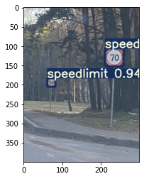

Apart from a folder of images, there are other sources we can use for our detector as well. These include http, rtsp, rtmp video streams, which can add a lot of utility to deploying such a model into production. The command syntax for doing so is described by the following.

python detect.py --source 0  # webcam
                            file.jpg  # image 
                            file.mp4  # video
                            path/  # directory
                            path/*.jpg  # glob
                            rtsp://170.93.143.139/rtplive/470011e600ef003a004ee33696235daa  # rtsp stream
                            rtmp://192.168.1.105/live/test  # rtmp stream
                            http://112.50.243.8/PLTV/88888888/224/3221225900/1.m3u8  # http stream

Computing the mean Average Precision (mAP) on the test dataset

We can use the  test.py  script to compute the mAP of the model predictions on our test set.  The script calculates for us the Average Precision for each class, as well as the mean Average Precision (mAP). To perform the evaluation on our test set, we need to set the task flag to test. We will then set the name to yolo_det. The various outputs of test.py, like plots of various curves (F1, AP, Precision curves etc), can then be found in the output folder: runs/test/yolo_road_det.

!python test.py --weights runs/train/yolo_road_det/weights/best.pt --data road_sign_data.yaml --task test --name yolo_det

The output of which looks like the following:

Fusing layers... 
Model Summary: 224 layers, 7062001 parameters, 0 gradients, 16.4 GFLOPS
test: Scanning 'Road_Sign_Dataset/labels/test' for images and labels... 
test: New cache created: Road_Sign_Dataset/labels/test.cache
test: Scanning 'Road_Sign_Dataset/labels/test.cache' for images and labels...
               Class      Images     Targets           P           R      mAP@.5
                 all          88         126       0.961       0.932       0.944         0.8
        trafficlight          88          20       0.969        0.75       0.799       0.543
                stop          88           7           1        0.98       0.995       0.909
          speedlimit          88          76       0.989           1       0.997       0.906
           crosswalk          88          23       0.885           1       0.983       0.842
Speed: 1.4/0.7/2.0 ms inference/NMS/total per 640x640 image at batch-size 32
Results saved to runs/test/yolo_det

Closing thoughts

With that, we have completed the tutorial. Readers of this tutorial should now be able to train YOLOv7 on any custom dataset, like the example used with road signs. While not all datasets will use this xml formatting, this system is robust enough to be applied to any object detection dataset to run with YOLOv7.

Be sure to try out this demo in a Gradient Notebook, and try scaling the GPU to higher VRAM enabled machines to see how that affects training times.

Credits to Ayoosh Kathuria for his excellent work on his original YOLOv5 tutorial, which we have adapted to YOLOv7 here. Please be sure to check out his other articles on the blog.

The github repo for this project may be found here.