Through a series of tutorials, the gradient descent (GD) algorithm will be implemented from scratch in Python for optimizing parameters of artificial neural network (ANN) in the backpropagation phase. The GD implementation will be generic and can work with any ANN architecture. The tutorials will follow a simple path to fully understand how to implement GD. Each tutorial will cover the required theories and then applies then in Python.

In this tutorial, which is the Part 1 of the series, we are going to make a worm start by implementing the GD for just a specific ANN architecture in which there is an input layer with 1 input and an output layer with 1 output. This tutorial will not use any hidden layers. For simplicity, no bias will be used at the beginning.

1 Input – 1 Output

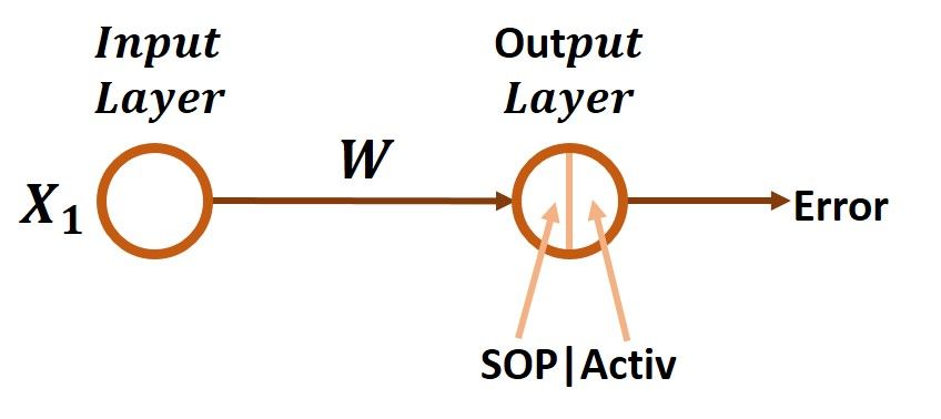
The first step towards the generic implementation of the GD algorithm is to implement it just for a very simple architecture as shown in the figure below. There are only 1 input and 1 output and no hidden layers at all. Before thinking of using the GD algorithm in the backward pass, let's start by the forward pass and see how we can move from the input until calculating the error.

Forward Pass

According to the below figure, the input X1 is multiplied by its weight W to return the result X1*W. In the forward pass, it is generally known that each input is multiplied by its associated weight and the products between all inputs and their weights are then summed. This is called the sum of products (SOP). For example, there are 2 inputs X1 and X2 and their weights are W1 and W2, respectively, then the SOP will be X1*W1+X2*W2. In this example, there is only 1 input and thus the SOP is meaningless.

After calculating the SOP, next is to feed it to the activation function in the output layer neuron. Such a function helps to capture the non-linear relationships between the inputs and the outputs and thus increasing the accuracy of the network. In this tutorial, the sigmoid function will be used. Its formula is given in the next figure.

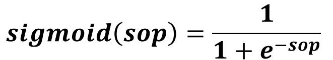
Assuming that the outputs in this example range from 0 to 1, then the result returned from the sigmoid could be regarded as the predicted output. This example is a regression example but it could be converted into a classification example easily by mapping the score returned by the sigmoid to a class label.

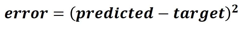
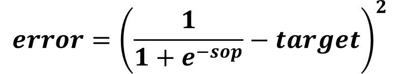
After calculating the predicted output, next is to measure the error of prediction using the square error function defined below.

At this time, the forward pass is complete. Based on the calculated error, we can go backward and calculate the weight gradient which is used for updating the current weight.

Backward Pass

In the backward pass, we are looking to know how the error changes by changing the network weights. As a result, we want to build an equation in which both the error and the weight exist. How to do that?

According to the previous figure, the error is calculated using 2 terms which are:

1. predicted
2. target

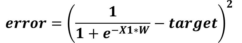
Do not forget that the predicted value is calculated as the output of the sigmoid function. Thus, we can substitute by the sigmoid function into the error equation and the result will be as given below. But up this point, the error and the weight are not included in this equation.

This is right but also remember that the sop is calculated as the product between the input X1 and its weight W. Thus, we can remove the sop and use its equivalent X1*W as given below.

At this time, we can start calculating the gradient of the error relative to the weight as given in the next figure. Using the equation below for calculating the gradient might be complex especially when more inputs and weights exist. As an alternative, we can use the chain rule which simplifies the calculations.

Chain Rule

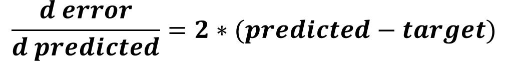
When the 2 participants of the gradient, which are the error and W in this example, are not related directly by a single equation, we can follow a chain of derivatives that starts from the error until reaching W. Looking back to the error function, we can find that the prediction is the link between the error and the weight. Thus, we can calculate the first derivative which is the derivative of the error to the predicted output as given below.

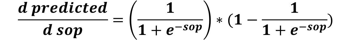
After that, we can calculate the derivative of the predicted to the sop by calculating the derivative of the sigmoid function according to the figure below.

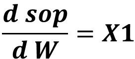
Finally, we can calculate the derivative between the sop and the weight as given in the next figure.

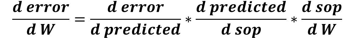
After going through the chain of derivatives, we can associate the error by the weight by multiplying all derivatives as given below.

Python Implementation

After understanding how the process work theoretically, we can apply it easily. The code listed below goes through the steps discussed previously.  The input X1 value is 0.1 and the target is 0.3. The weight is initialized randomly using numpy.random.rand()which returns a number between 0 and 1. After that, input and weight are propagated into the forward pass. This is by calculating the product between the input and the weight and then calling the sigmoid() function. Remember that the output from the sigmoid() function is regarded as the predicted output. After calculating the predicted output, the final step is to calculate the error using the error() function. By doing that, the forward pass is complete.

import numpy


def sigmoid(sop):
    return 1.0 / (1 + numpy.exp(-1 * sop))


def error(predicted, target):
    return numpy.power(predicted - target, 2)


def error_predicted_deriv(predicted, target):
    return 2 * (predicted - target)


def activation_sop_deriv(sop):
    return sigmoid(sop) * (1.0 - sigmoid(sop))


def sop_w_deriv(x):
    return x


def update_w(w, grad, learning_rate):
    return w - learning_rate * grad


x = 0.1
target = 0.3
learning_rate = 0.001
w = numpy.random.rand()
print("Initial W : ", w)

# Forward Pass
y = w * x
predicted = sigmoid(y)
err = error(predicted, target)

# Backward Pass
g1 = error_predicted_deriv(predicted, target)

g2 = activation_sop_deriv(predicted)

g3 = sop_w_deriv(x)

grad = g3 * g2 * g1
print(predicted)

w = update_w(w, grad, learning_rate)

In the backward pass, the derivative of the error to the predicted output is calculated using the error_predicted_deriv()function and the result is stored in the variable g1. After that, the derivative of the predicted (activation) output to the sop is calculated using the activation_sop_deriv() function. The result is stored in the variable g2. Finally, the derivative of the sop to the weight is calculated using the sop_w_deriv() function and the result is stored in the variable g3.

After calculating all derivatives in the chain, next is to calculate the derivative of the error to the weight by multiplying all derivatives g1, g2, and g3. This returns the gradient by which the weight value could be updated. The weight is updated using the update_w() function. It accepts 3 arguments:

1. w
2. grad
3. learning_rate

This returns the updated weight which replaces the old one. Note that the previous code does not repeat re-train the network using the updated weight. We can go through several iterations in which the gradient descent algorithm can reach a better value for the weight according to the modified code below. Note that you can change the learning rate and the number of iterations until making the network make correct predictions.

import numpy

def sigmoid(sop):
    return 1.0 / (1 + numpy.exp(-1 * sop))

def error(predicted, target):
    return numpy.power(predicted - target, 2)

def error_predicted_deriv(predicted, target):
    return 2 * (predicted - target)

def activation_sop_deriv(sop):
    return sigmoid(sop) * (1.0 - sigmoid(sop))

def sop_w_deriv(x):
    return x

def update_w(w, grad, learning_rate):
    return w - learning_rate * grad

x = 0.1
target = 0.3
learning_rate = 0.01
w = numpy.random.rand()
print("Initial W : ", w)

for k in range(10000):
    # Forward Pass
    y = w * x
    predicted = sigmoid(y)
    err = error(predicted, target)

    # Backward Pass
    g1 = error_predicted_deriv(predicted, target)

    g2 = activation_sop_deriv(predicted)

    g3 = sop_w_deriv(x)

    grad = g3 * g2 * g1
    print(predicted)

    w = update_w(w, grad, learning_rate)

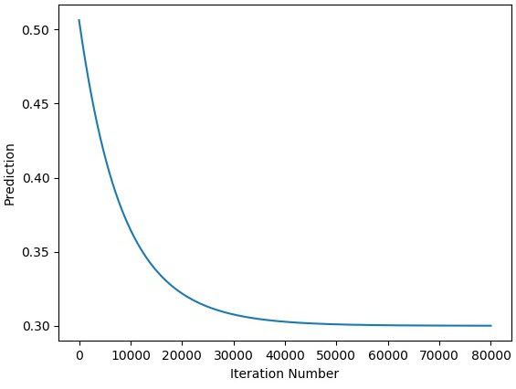
The next figure shows how the network prediction enhances by iterations. The network can reach the desired output after 50000 iterations. Note that you can reach the desired output by less number of iterations by changing the learning rate.

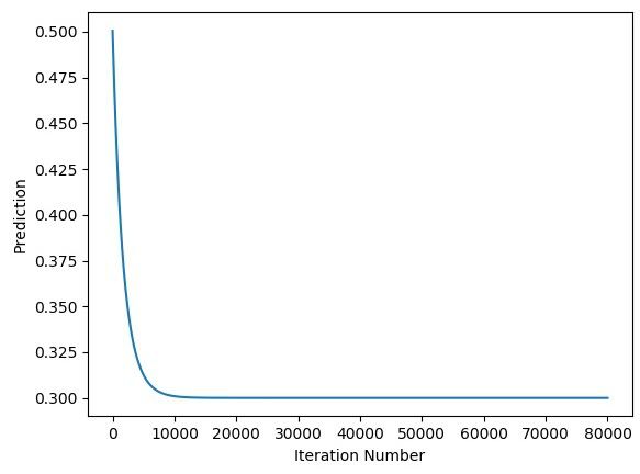
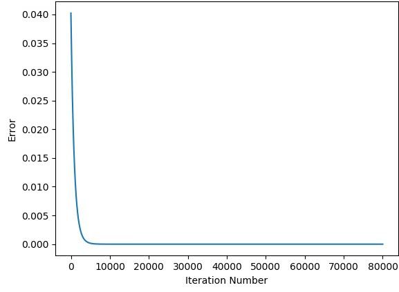
When the learning rate is 0.5, the network reached the desired output after only 10000 iterations.

The next figure shows how the network error changes by iteration when the learning rate is 0.5.

After building the GD algorithm which can work effectively for the basic architecture with 1 input and 1 output, we can increase the number of inputs from 1 to 2 in the next section. Note that it is very important to understand how the previous implementation works because the next sections will be highly dependent on it.

Conclusion

Up to this point, we successfully implemented the GD algorithm for working with either 1 input or 2 inputs. In the next tutorial, the previous implementation will be extended to allow the algorithm to work with more inputs. Using the examples that will be discussed in the next tutorial, a general rule will be derived for allowing the GD algorithm to work with any number of inputs.