
Introduction
In this ever-evolving field of computer vision, the emergence of Vision Transformers (ViTs) has been a groundbreaking concept. These models, introduced by Dosovitskiy et al. in the paper "An Image is Worth 16x16 Words: Transformers for Image Recognition (2020)," have proven a noted improvement and replacement to traditional convolutional neural network (CNN) approaches. ViTs offers a novel Transformer architecture that leverages the attention mechanism for image analysis.
As the demand for advanced computer vision systems continues to surge across various industries, the deployment of Vision Transformers has become a focal point for researchers and practitioners. However, harnessing the full potential of these models requires a deep understanding of their architecture. Also, it is equally crucial to develop an optimization strategy for an efficient deployment of these models.
This article aims to provide an overview on Vision Transformers, a comprehensive exploration of their architecture, key components, and the underlying principles that sets them apart. At the end of the article, we will discuss a few of the optimization strategies to make the model more compact for deployment with a code demo.
Overview of Transformer Models
ViTs are a special type of neural network that finds its major application in image classification and object detection. The accuracy of ViTs have surpassed traditional CNNs, and a key factor contributing to this is their foundation on the Transformer architecture. Now what is this architecture?
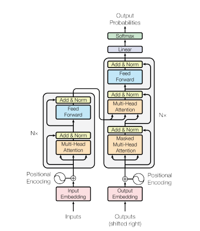
In 2017, the Transformer neural network architecture was introduced in the paper "Attention is all you need" by Vaswani et al. This network utilizes an encoder and a decoder structure very similar to a Recurrent Neural Network (RNN). In this model, there are no notion of timestamps for the input; all words are passed simultaneously, and their word embeddings are determined concurrently.
This type of neural network architecture relies on a mechanism called self-attention.
Here's a high-level explanation of the key components of the Transformer architecture:
- Input-Embeddings: Input-Embedding is the first step to pass the input to the transformers. Input embedding refers to the process of converting input tokens or words into fixed-size vectors that can be fed into the model. This embedding step is crucial because it transforms the discrete token representations into continuous vector representations in a way that captures semantic relationships between words. This embedding step maps a word to a vector, but the same word with different sentences may have different meanings. This is were positional encoders comes in.
- Positional Encodings: Since Transformers do not inherently understand the order of the elements in a sequence, positional encodings are added to the input embeddings to give the model information about the positions of elements in the sequence. In simpler terms, the positional embeddings gives a vector which is context based on position of the word in a sentence. The original paper uses a sin and cosine function to generate this vector. This information is passed to the encoder block.
- Encoder-Decoder Structure: The Transformer is primarily used for sequence-to-sequence tasks, like machine translation. It consists of an encoder and a decoder. The encoder processes the input sequence, and the decoder generates the output sequence.
- Multi-Head Self-Attention: Self-attention allows the model to weigh different parts of the input sequence differently when making predictions. The key innovation in the Transformer is the use of multiple attention heads, allowing the model to focus on different aspects of the input simultaneously. Each attention head is trained to attend to different patterns.
- Scaled Dot-Product Attention: The attention mechanism computes a set of attention scores by taking the dot product of the input sequence with learnable weight vectors. These scores are scaled and passed through a softmax function to obtain attention weights. The weighted sum of the input sequence using these attention weights is the output of the attention mechanism.
- Feedforward Neural Networks: After attention layers, each encoder and decoder block typically includes a feedforward neural network with an activation function such as ReLu. This network is applied independently to each position in the sequence.
- Layer Normalization and Residual Connections: Layer normalization and residual connections are used to stabilize training. Each sub-layer (attention or feedforward) in the encoder and decoder has layer normalization, and the output of each sub-layer is passed through a residual connection.
- Encoder and Decoder Stacks: The encoder and decoder are composed of multiple identical layers stacked on top of each other. The number of layers is a hyperparameter.
- Masked Self-Attention in Decoders: During training, in the decoder, the self-attention mechanism is modified to prevent attending to future tokens. This is done using a masking technique to ensure that each position can only attend to positions before it.
- Final Linear and Softmax Layer: The output of the decoder stack is transformed into the final predicted probabilities (e.g., using a linear layer followed by a softmax activation) for generating the output sequence.
Understanding Vision Transformer Architecture
CNNs were considered to be the best solutions for image classification tasks. ViTs consistently beat CNNs on such tasks, if the dataset for pre-training is sufficiently large. ViTs have marked a significant achievement by successfully training a Transformer encoder on ImageNet, showcasing impressive results in comparison to well-known convolutional architectures.
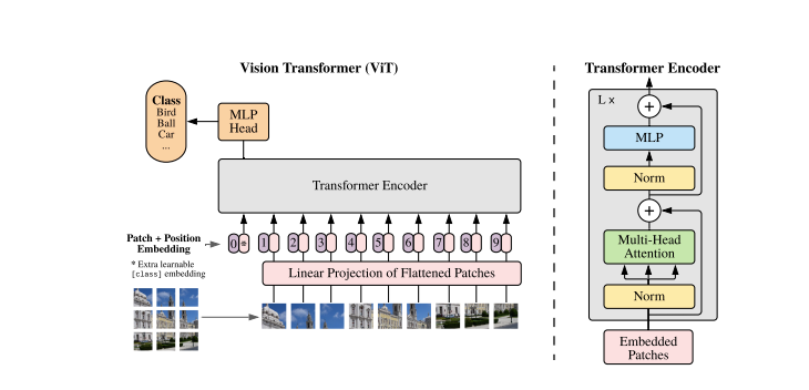
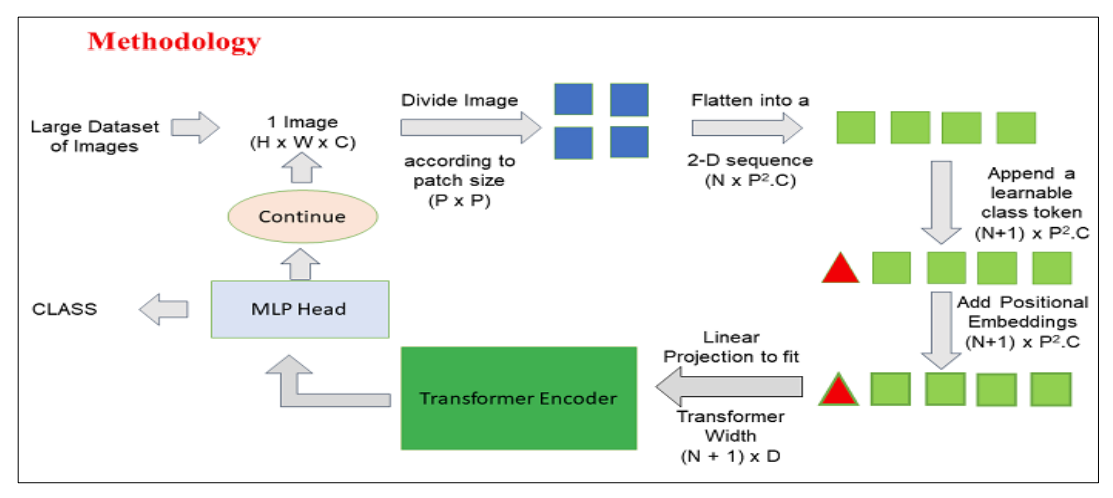
Transformers models typically work with images and words that are passed in sequence to the encoder-decoder. Here is a simplified overview of ViTs:
- Patch Extraction: The images, as sequences of patches are fed to the Transformer encoder. A patch refers to a small rectangular section within an image, typically measuring 16x16 pixels in size.

- After dividing the image into non-overlapping patches (typically 16x16 grid), each patch is transformed into a vector that represents its features. These features are usually extracted through the utilization of a convolutional neural network (CNN), which is trained to identify significant characteristics essential for image classification.
- Linear Embedding: These extracted patches are linearly embedded into flat vectors. These vectors are then treated as the input sequence for the Transformer a.ka.a Linear Projection of Flattened Patches.
- Transformer Encoder: The embedded patch vectors are passed through a stack of Transformer encoder layers. Each encoder layer consists of self-attention mechanisms and feedforward neural networks.
- Self-Attention Mechanism: The self-attention mechanism allows the model to capture relationships between different patches in the image, enabling it to learn long-range dependencies and relationships. The attention mechanism in the Transformer allows the model to capture both local and global contextual information, making it effective for a wide range of vision tasks.
- Positional Encoding: Since the Transformer does not inherently understand the spatial relationships between patches, positional encodings are added to the input embeddings to provide information about the patch positions in the original image.
- Multiple Encoder Layers: The ViTs typically uses multiple Transformer encoder layers to capture hierarchical and abstract features from the input image.
- Global Average Pooling: The output of the Transformer encoder is often subjected to global average pooling, which aggregates the information from different patches into a fixed-size representation.
- Classification Head: The pooled representation is then fed into a classification head, typically consisting of one or more fully connected layers, to produce the final output for the specific computer vision task (e.g., image classification).
We highly recommend checking out the original research paper for a deeper understanding of ViTs architecture.
How to use
Bring this project to life
Here is python demo on how to use this model to classify an image:
#install the transformers libraries using pip
!pip install -q transformers
Import the necessary classes from the Transformer library. ViTFeatureExtractor is used for extracting features from images, and ViTForImageClassification is a pre-trained ViT model for image classification.
from transformers import ViTFeatureExtractor, ViTForImageClassification
from PIL import Image as img
from IPython.display import Image, display

#specify the path to image
FILE_NAME = '/notebooks/football-1419954_640.jpg'
display(Image(FILE_NAME, width = 700, height = 400))

How to use a pre-trained Vision Transformer (ViT) model to predict the class of an input image.
image_array = img.open('/notebooks/football-1419954_640.jpg')

#loading the ViT Feature Extractor and Model
feature_extractor = ViTFeatureExtractor.from_pretrained('google/vit-base-patch16-224')
model = ViTForImageClassification.from_pretrained('google/vit-base-patch16-224')

#Extracting Features and Making Predictions:
inputs = feature_extractor(images = image_array,
                           return_tensors="pt")
outputs = model(**inputs)
logits = outputs.logits

# model predicts one of the 1000 ImageNet classes
predicted_class_idx = logits.argmax(-1).item()
print(predicted_class_idx)
#805
print("Predicted class:", model.config.id2label[predicted_class_idx])
#Predicted class: soccer ball
Here is code breakdown:
ViTFeatureExtractor.from_pretrained: This is responsible for converting the input image into a format suitable for the ViT model.ViTForImageClassification.from_pretrained: Loads a pre-trained ViT model for image classification.feature_extractor: Processes the input image using the ViT feature extractor, converting it into a format suitable for the ViT model.model: Pre-trained model processes the input and produces output logits, representing the model's predictions for different classes.- The next steps is followed by finding the index of the class with the highest logit score. Creating a variable that stores the index of the predicted class.
model.config.id2label[predicted_class_idx]: Maps the predicted class index to its corresponding label.
Originally, the ViT model was pre-trained using the famous ImageNet-21k, a dataset consisting of 14 million images and 21k classes, and was fine-tuned on ImageNet dataset which includes 1 million images and 1k classes.
Optimization Strategies
ViTs report an outstanding performance in tasks such as image classification, object detection, and semantic segmentation. Furthermore, the Transformer architecture itself has demonstrated performance improvements over CNN. However these architectures require massive amounts of data to train and high computational resources. Due to this the models deployment becomes heavy.
Model compression has become a new point of research, offering a promising solution to address the challenges of resource-intensive models. Various techniques have emerged in the literature to compress models, including weight quantization, weight multiplexing, pruning, and Knowledge Distillation (KD). Knowledge distillation (KD) has proven to be a straightforward yet highly efficient method for compressing models. It enables a less intricate model to achieve task performance nearly on par with the original model.
Knowledge distillation is a model compression technique in machine learning where a complex model, often referred to as the "teacher" model, transfers its knowledge to a simpler model, known as the "student" model. The goal is to distill the essential information or knowledge learned by the teacher model into the student model, allowing the student model to achieve similar performance on a given task. This process typically involves training the student model to mimic the output probabilities or representations of the teacher model, helping to reduce the computational resources required while maintaining satisfactory performance.
Several distilled model approaches have proven to be effective for ViT compression such as Target aware Transformer, Fine-Grain Manifold Distillation Method, Cross Inductive Bias Distillation (Coadvice), Tiny-ViT, Attention Probe-based Distillation Method, Data-Efficient Image Transformers Distillation via Attention (DeiT), Unified Visual Transformer Compression (UVC), Dear-KD Distillation Method, Cross Architecture Distillation Method, and many more.
What is DeiT
A novel technique in the field of vision transformers was developed by Touvron et al. named Training Data-Efficient Image Transformers Distillation via Attention a.k.a. DeiT. DEiT, or Data-efficient Image Transformer, is a type of vision transformer that addresses the challenge of training large-scale transformer models on limited labeled data. Vision transformers have gained attention for their success in computer vision tasks, but training them often requires extensive labeled datasets and computing resources.
DeiT is a convolution-free transformer which is exclusively trained on the ImageNet dataset. The training process took less than three days on a single computer. The benchmark model was a vision transformer, consisting of 86 million parameters.
DeiT is introduced as the teacher-student strategy and relies on KD ensuring the student learns from the teacher model through attention. The main idea is to pre-train a large teacher model on a large dataset (e.g., ImageNet) where abundant labeled examples are available. The knowledge learned by this teacher model is then transferred to a smaller student model, which is trained on the target dataset with limited labeled samples.
| Vit | DeiT |
|---|---|
| Training required massive dataset which is not available publicly as well | Trained only using ImageNet 10 times smaller dataset |
| Trained using extensive compute power, also the training time was longer | Trained using a single computer in less than 3 days, with a single 8 GPU or 4GPU machine |
| Required 300 M samples dataset | 30 M samples dataset |
Apart from KD, DeiT requires a knowledge of Regularization and Data Augmentation. In simpler terms regularization prevents the model from overfitting to the training data, it helps the model to learn the actual information from the data. Augmentation refers to the technique of artificially increasing the size of a dataset by applying various transformations to the existing data. This helps in getting different variations of the same data. These are the among the few major techniques used in DeiT, however the major contributor was KD.
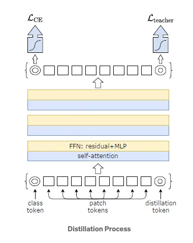
In the original research paper, DeiT proposes a modified approach of KD also known as Hard Distillation. Here the teacher network is the state of the art CNN pretrained on ImageNet. The Student network is the modified version of transformer. The main modification is the output of the CNN is further passed as an input to the transformer.
- Hard Decision of the teacher network is the true label, the goal associated to this hard-label distillation is:

- New distillation tokens are introduced along with the class tokens and patch tokens. These tokens interacts with the other two through self-attention layers.
- In all subsequent distillation experiments, the default teacher is a RegNetY-16GF with 84 million parameters. The experiments employ the same dataset and data augmentation as DeiT.
- DeiT Architecture variations:
- DeiT-Ti: Tiny model with 5M parameters
- DeiT-S: Small model with 22M parameters
- DeiT-B: Large model with 86M parameters
- DeiT-b 384: Fine tuned model for larger resolution of 384x384
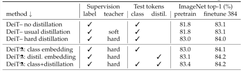
- DeiT: Uses distillation process
In the image below, we can assess the efficacy of hard distillation, as the accuracy reaches nearly 83%, a level unattainable through soft distillation. Additionally, the distillation tokens brings slightly better results.
- Training DeiT-B for 300 epochs typically requires 37 hours on 2 nodes or 53 hours on a single 8-GPU node.
A Code Demo and In-Depth Understanding for Efficient Deployment
Bring this project to life
DeiT demonstrates the successful application of Transformers in computer vision tasks, even with limited data availability and resources.
Classifying Images with DeiT
Please refer to the detailed instructions in the README.md of the DeiT repository for guidance on image classification using DeiT. Alternatively, for a quick test, begin by installing the necessary packages:
!pip install torch torchvision timm pandas requests
Next, run the below script
from PIL import Image
import torch
import timm
import requests
import torchvision.transforms as transforms
from timm.data.constants import IMAGENET_DEFAULT_MEAN, IMAGENET_DEFAULT_STD

print(torch.__version__)
# should be 1.8.0


model = torch.hub.load('facebookresearch/deit:main', 'deit_base_patch16_224', pretrained=True)
model.eval()

transform = transforms.Compose([
    transforms.Resize(256, interpolation=3),
    transforms.CenterCrop(224),
    transforms.ToTensor(),
    transforms.Normalize(IMAGENET_DEFAULT_MEAN, IMAGENET_DEFAULT_STD),
])

img = Image.open(requests.get("https://images.rawpixel.com/image_png_800/czNmcy1wcml2YXRlL3Jhd3BpeGVsX2ltYWdlcy93ZWJzaXRlX2NvbnRlbnQvcHUyMzMxNjM2LWltYWdlLTAxLXJtNTAzXzMtbDBqOXFrNnEucG5n.png", stream=True).raw)
img = transform(img)[None,]
out = model(img)
clsidx = torch.argmax(out)
print(clsidx.item())
Now, this should output 285, which, according to the list of classes from the ImageNet index (labels file), maps to 'Egyptian cat.'
This code essentially demonstrates how to use a pre-trained DeiT model for image classification and prints the output that is the index of the predicted class. Let us understand the code briefly by breaking it down further.
- Installing Libraries: The first necessary step is installing the required libraries. We highly recommend the users to research on the libraries for a better understanding.
- Loading Pre-trained Model:
model = torch.hub.load('facebookresearch/deit:main', 'deit_base_patch16_224', pretrained=True): Loads a pre-trained DeiT model named 'deit_base_patch16_224' from the DeiT repository. - Setting Model to Evaluation Mode:
model.eval(): Sets the model to evaluation mode, which is important when using a pre-trained model for inference. - Image Transformation: Defines a series of transformation to be applied to the image. Such as resizing, center cropping, converting the image to PyTorch tensor, normalize the image using the mean and standard deviation values commonly used for ImageNet data.
- Downloading and transforming the image: The next step involves downloading the image from a URL and transforming it. Adding the parameter
[None,]adds an extra dimension to simulate a batch of size 1. - Model Inference and prediction:
out = model(img)will allow the preprocessed image through the DeiT model for inference.clsidx = torch.argmax(out)will find the index of the class with the highest probability. Next, print the index of the predicted class.
Quantizing the model
To reduce the model size, quantization is applied. This process reduces the size by not hampering the model accuracy.
#Specifies the quantization backend as "qnnpack." QNNPACK (Quantized Neural Network PACKage) is a library for low-precision quantized neural network inference developed by Facebook

backend = "qnnpack"

model.qconfig = torch.quantization.get_default_qconfig(backend)
torch.backends.quantized.engine = backend

quantized_model = torch.quantization.quantize_dynamic(model, qconfig_spec={torch.nn.Linear}, dtype=torch.qint8)

scripted_quantized_model = torch.jit.script(quantized_model)
scripted_quantized_model.save("fbdeit_scripted_quantized.pt")
In summary, this code snippet quantizes the model, and saves the model to a file named "fbdeit_scripted_quantized.pt." The most important part of the code is explained below:
torch.quantization.quantize_dynamic(model, qconfig_spec={torch.nn.Linear}, dtype=torch.qint8): It quantizes the weights of the model during the inference process, and qconfig_spec specifies that quantization should be applied only to linear (fully connected) layers. The quantized data type used is torch.qint8 (8-bit integer quantization).
Optimizing the model
To optimize the model more run the below code snippet:
from torch.utils.mobile_optimizer import optimize_for_mobile
optimized_scripted_quantized_model = optimize_for_mobile(scripted_quantized_model)
optimized_scripted_quantized_model.save("fbdeit_optimized_scripted_quantized.pt")
out = optimized_scripted_quantized_model(img)
clsidx = torch.argmax(out)
print(clsidx.item())In this code snippet takes a scripted and quantized model, optimizes it specifically for mobile deployment using the optimize_for_mobile function, and saves the resulting optimized model to a file. The optimization aims to make the model more efficient in terms of both memory usage and inference speed, which is crucial for running models on resource-constrained mobile devices.
optimized_scripted_quantized_model = optimize_for_mobile(scripted_quantized_model): The optimize_for_mobile function performs various optimizations for mobile deployment, such as reducing the model's memory footprint and improving inference speed. The result is an optimized version of the scripted and quantized model.
The Lite version
Let’s create the lite version of the model.
optimized_scripted_quantized_model._save_for_lite_interpreter("fbdeit_optimized_scripted_quantized_lite.ptl")
ptl = torch.jit.load("fbdeit_optimized_scripted_quantized_lite.ptl")
This process is important for deploying models on mobile or edge devices that support PyTorch Lite, ensuring compatibility and efficiency in the runtime environment of such devices.
Comparing Inference Speed
To compare the different model variations in terms of inference speed execute the provided code.
with torch.autograd.profiler.profile(use_cuda=False) as prof1:
    out = model(img)

with torch.autograd.profiler.profile(use_cuda=False) as prof2:
    out = scripted_quantized_model(img)

with torch.autograd.profiler.profile(use_cuda=False) as prof3:
    out = optimized_scripted_quantized_model(img)

with torch.autograd.profiler.profile(use_cuda=False) as prof4:
    out = ptl(img)

print("original model: {:.2f}ms".format(prof1.self_cpu_time_total/1000))

print("scripted & quantized model: {:.2f}ms".format(prof2.self_cpu_time_total/1000))

print("scripted & quantized & optimized model: {:.2f}ms".format(prof3.self_cpu_time_total/1000))

print("lite model: {:.2f}ms".format(prof4.self_cpu_time_total/1000))
We strongly advise clicking the provided link in this article to access the complete code within the Paperspace notebook.
Concluding Thoughts
In this article we have included everything to get started with vision transformer and explore this model using the Paperspace console. We have explored one of the important applications for the model: image recognition. We have also included Transformer architecture for the sake of comparison and easier interpretation of ViT.
The Vision Transformer paper, introduced a promising and straightforward model as a replacement for CNNs. This model attained state-of-the-art benchmarks on popular image classification datasets, including Oxford-IIIT Pets, Oxford Flowers, and Google Brain's JFT-300M, following pre-training on ILSVRC's ImageNet and its superset ImageNet-21M.
In conclusion, Vision Transformers (ViTs) and the DeiT represent significant advancements in the field of computer vision. ViTs, with their attention-based architecture, demonstrated the effectiveness of transformer models in image understanding, challenging traditional convolutional approaches.
DeiT, in particular, further addressed the challenges faced by ViT by introducing knowledge distillation. By leveraging a teacher-student training paradigm, DeiT showcased the potential to achieve competitive performance with significantly less labeled data, making it a valuable solution in scenarios where large datasets are not readily available.
As research in this area continues to evolve, these innovations pave the way for more efficient and powerful models, promising exciting possibilities for the future of computer vision applications.
References
- Vision Transformers Explained
- An image is worth 16x16 words: Transformers from image recognition at scale
- Knowledge Distillation in Vision Transformers: A Critical Review
- Training data-efficient image transformers & distillation through attention
- Detailed Explanation on DeiT
- Vision Transformer (ViT): Hugging Face Overview
- QNNPACK: Open source library for optimized mobile deep learning
- Code reference: https://pytorch.org/tutorials/beginner/vt_tutorial.html#using-lite-interpreter