A Review of the Image Quality Metrics used in Image Generative Models

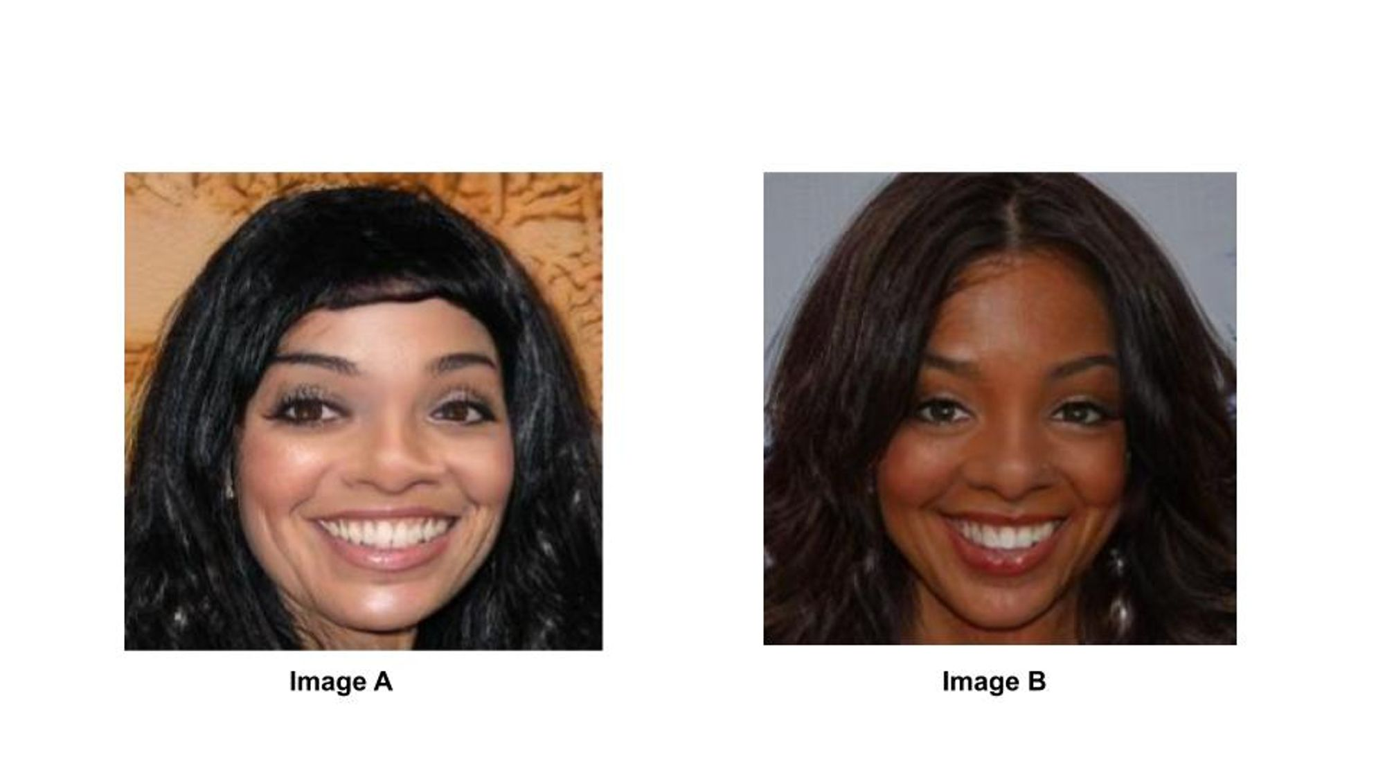
We know that machine learning is a subfield of artificial intelligence in which we train computer algorithms to learn patterns in the training data in order to make decisions on unseen data. Machine learning has paved the way for tasks like image classification, object detection and segmentation within images, and recently image generation. The task of image generation falls under the creative aspect of computer vision. It involves creating algorithms that synthesize image data that mimics the distribution of real image data that a machine learning model was trained on. Image generation models are trained in an unsupervised fashion which leads to models that are highly skewed toward discovering patterns in the data distribution without the need to consider a right or wrong answer. As a result of this, there is no particular correct answer, or in this case image, when it comes to evaluating the generated images. As humans, we have an inherent set of rules that we can use to evaluate the quality of an image. If I presented the two images below and asked you, “Which of these images looks better?”, you would respond by saying “A” or “B” based on the different appeals of each image.

Suppose I asked you, “Which of the images below looks more realistic?” You would select  “A” or “B”  based on whichever image reminded you more of someone or something you have seen before in real life.

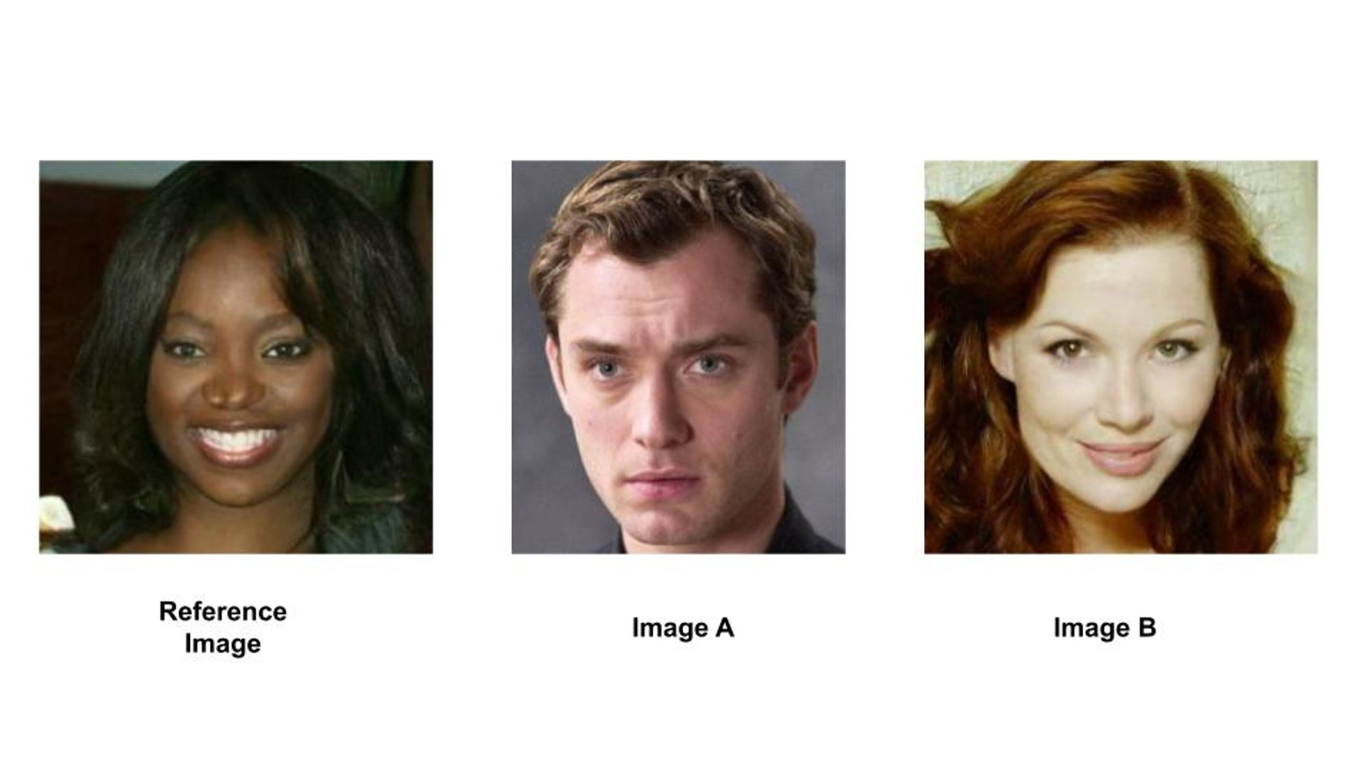
For the final question I could ask, “Which of these images appears to be more similar to the reference image?”. Again you would respond by saying “A” or “B” based on what you deemed as the most important aspects of the reference image and finding the image with the least differences along those very aspects.

In all of the questions above I have asked about the independent image quality, the image quality with respect to the real world, and the image quality with respect to a reference. These are the 3 different aspects that researchers consider when trying to evaluate the correctness of generated images. While answering the questions above you might have thought about various image features when selecting your chosen answer. It might have been variations in light intensity, the sharpness or lack thereof of the lines, the symmetry in the content objects, or the blurriness of the object backgrounds. All of these are valid features to point out while highlighting image similarity or dissimilarity. As humans we can use natural language to communicate, “that picture looks way off” or “the texture on that person’s skin looked eerie”. When it comes to computer vision algorithms, we need a method to quantify the differences between generated images and real images in a way that corresponds with human judgment. In this article, I will highlight some of these metrics that are commonly used in the field today.

Note: I assume that the audience has a high-level familiarity with generative models.

CONTENT VARIANT METRICS

These are metrics that are useful when the generated image can take different content objects per input noise vector. This means that there is no right answer.

Inception Score (IS)

The inception score is a metric designed to measure the image quality and diversity of generated images. It was initially created as an objective metric for generative adversarial networks (GAN). In order to measure the image quality, generated images are fed into a pretrained image classifier network in order to obtain the probability score for each class. If the probability scores are widely distributed then the generated image is of low quality. The intuition here is that if there is a high probability that the image could belong to multiple classes, then the model cannot clearly define what object is contained in the image. A wide probability distribution is commonly referred to as “high entropy”. What we aim for is low entropy. In the original paper, the generated images are fed into a pretrained image classifier network (InceptionNet) which was trained on the CIFAR10 dataset.

$entropy = -\sum(p_i\cdot log(p_i))$

Frechet Inception Distance (FID)

Unlike the Inception Score, the FID compares the distribution of generated images with the distribution of real images. The first step involves calculating the feature vector of each image in each domain using the InceptionNet v3 model which is used for image classification. FID compares the mean and standard deviation of the gaussian distributions containing feature vectors obtained from the deepest layer in Inception v3. High-quality and highly realistic images tend to have low FID scores meaning that their low dimension feature vectors are more similar to those of real images of the same type e.g faces to faces, birds to birds, etc. The calculation is:

$d^2 = ||\mu_1-\mu_2||^2 + Tr(C_1 + C_2 - 2\sqrt{C_1\cdot C_2})$

Machine Learning Mastery did a great job explaining the different terms:

• The “mu_1” and “mu_2” refer to the feature-wise mean of the real and generated images, e.g. 2,048 element vectors where each element is the mean feature observed across the images.
• The C_1 and C_2 are the covariance matrix for the real and generated feature vectors, often referred to as sigma.
• The ||mu_1 – mu_2||^2 refers to the sum squared difference between the two mean vectors. Tr refers to the trace linear algebra operation, e.g. the sum of the elements along the main diagonal of the square matrix.
• The sqrt is the square root of the square matrix, given as the product between the two covariance matrices.

The authors of the original paper proved that FID was superior to the inception score because it was more sensitive to subtle changes in the image i.e. gaussian blur, gaussian blur, salt & pepper noise, ImageNet contamination

CONTENT INVARIANT METRICS

These are metrics that are best used when there is only one correct answer for the content in the images.  An example of a model that uses these metrics is a NeRF model which generates viewpoints for different viewpoints. For each viewpoint, there is only one acceptable perception of the objects in the scene. Using content invariant metrics you can tell whether an image has noise that prevents it from looking like the ground truth image.

Learned Perceptual Image Patch Similarity (LPIPS)

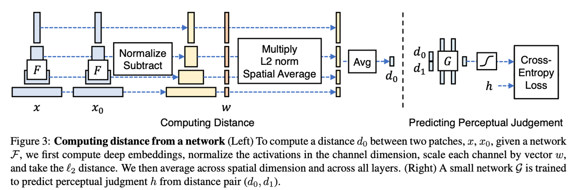
This is another objective metric for calculating the structural similarity of high-dimensional images whose pixel values are contextually dependent on one another. Like FID, LPIPS takes advantage of internal activations of deep convolutional networks because of their useful representational ability for low-dimension vectors. Unlike previous metrics, LPIPS measures perceptual similarity as opposed to quality assessment. LPIPS measures the distance in VGGNet feature space as a “perceptual loss” for image regression problems.

In order to use the deep features of a network to find the distance $d_o$ between a reference $x$ and 2 distorted patches $x_0, x_1$ given a network $F$  the authors employ the following steps:

• compute deep embeddings by passing $x$ into $F$
• normalize the activations in the channel dimension
• scale each channel by vector $w$
• take the $l_2$ distance

Structured Similarity Index Metric (SSIM, MSSIM)

L2 Distance uses pixel differences to measure the structural differences between two images (sample and reference). In order to outdo previous methods, the authors created a metric that mimicked the human visual perception system which is highly capable of identifying structural information from a scene. The SSIM metric identifies 3 metrics from an image: Luminance $l(x,y)$ , Contrast $c(x,y)$, and Structure $s(x,y)$. The specifics on how to calculate the 3 individual metrics is here

$SSIM(x,y) = [l(x,y)]^{\alpha}\cdot[c(x,y)]^\beta\cdot[s(x,y)]^\gamma$

where $\alpha>0, \beta> 0, \gamma>0$ denote the relative importance of each of the metrics to simplify the expression

Instead of taking global measurements of the whole image some implementations of SSIM take measurements of regions of the image and then average out the scores. This method is known as Mean Structural Similarity Index (MSSIM) and has proven to be more robust.

$MSSIM(X,Y) = \frac{1}{M}\sum_{j=1}^{M}SSIM(x_j,y_j)$

Peak Signal-to-Noise Ratio (PSNR)

“Signal-to-noise ratio is a measure used in science and engineering that compares the level of a desired signal to the level of background noise. SNR is defined as the ratio of signal power to noise power, often expressed in decibels. A ratio higher than 1:1 indicates more signal than noise” (Wikipedia) PSNR is commonly used to quantify reconstruction quality for images and videos subject to lossy compression.

PSNR is calculated using the mean squared error (MSE) or L2 distance as described below:

$PSNR = 20 \cdot log_{10}( MAX_I) - 10 \cdot log_{10}(MSE)$

$MAX_I$ is the maximum possible pixel value of the image. a higher PSNR generally indicates that the reconstruction is of higher quality

Bringing it all together

Content variant metrics have the capacity to evaluate the similarity/dissimilarity of images whose content differs because they utilize deep feature representations of the images. The essence of these vectors is that they numerically tell us the most important features associated with a sample image. Inception Score answers the question “How realistic is this image relative to the pretrained model?” because it evaluates the conditional probability distribution which only factors in the training data, the original number of classes, and the ability of the Inception V3 model.

FID is more versatile and asks the question, “How similar is this group of images relative to this other group of images?” FID takes the deepest layer of the inception v3 model as opposed to the classifier output as in Inception Score. In this case, you are not bound by the type and number of classes of the classifier. While analyzing the FID formula, I realized that averaging the feature vectors to get the sum squared distance in  $||\mu_1-\mu_2||^2$ means that FID will likely be skewed if the distribution of any group (1 or 2) is too wide. For instance, if you are comparing images of fruits and both your ground-truth and generated datasets have a disproportionately large amount of orange pictures relative to the other fruits, then FID is unlikely to highlight poorly generated strawberries and avocados. FID is plagued with the majority rules issue when it comes to domains with high variation. Now fruits are trivial, but what happens when you are looking at people's faces or cancer tumors?

The LPIPS metric is at the border of these content variant/invariant metrics because on one hand it uses deep features and could be considered almost a regional FID metric but it was designed for the purpose of assessing structural similarity in “same content-based“ images. LPIPS answers the question, “Did the structure of this patch change, and by how much?” While I might be tempted to believe that this metric might be able to give us a fine-grained version of the FID score, I’m afraid that my experiments from UniFace show that even with great variations of FID the LPIPS score shows very little variation. Additionally, while LPIPS mentions that their patch-wise implementation mirrors the patchwise implementation of convolution, LPIPS does not merge the output features of the patches of an image as does the convolution task with the feature vectors that are output. In this regard, LPIPS loses the global context of the input image which FID captures.

On the other hand, content invariant metrics are best when used on images with the same object content. We have seen from the different metrics above that some metrics measure structural differences between images on a pixel-wise basis (PSNR, SSIM, MSSIM) while others do so on a deep feature vector basis (LPIPS). In both of these cases, the metrics involved are evaluating images that have noise added to images that have a corresponding “clean” identical version. These metrics can be used for supervised learning tasks because a ground truth exists. These metrics answer the question, “How noisy is this generated image as compared to the ground truth image?”

In pixel-wise metrics like PSNR, SSIM, & MSSIM, the metrics assume pixel independence which means that they do not consider the context of the image. It would make sense to use these metrics when comparing two images with the same object contents in which one has some gaussian noise, but not two images of relatively similar images e.g two different pictures of a lion in the Sahara.

So why did I include these metrics if they aren’t useful for most content variant generative models? Because they are used to train NERF models to synthesize images of objects from different viewpoints. NERFs learn on a static set of input images and their corresponding views and then once trained, the NERF can synthesize an image from a new viewpoint without access to the ground-truth image (if any).

Concluding thoughts

In summary, we can use the metrics above to answer the following questions about two groups of images:

Inception Score: “How realistic is this image relative to the pretrained model?”

FID Score: “How similar is this group of images relative to this other group of images?”

LPIPS Score: “Did the structure of this patch change, and by how much?”

SSIM, MSSIM, PSNR: “How noisy is this generated image as compared to the ground truth image?”

The utility of these metrics will vary based on the nature of the task you are handling.

CITATIONS:

• Salimans, Tim, et al. "Improved techniques for training gans." Advances in neural information processing systems 29 (2016).APA
• Zhang, Richard, et al. "The unreasonable effectiveness of deep features as a perceptual metric." Proceedings of the IEEE conference on computer vision and pattern recognition. 2018.
• Heusel, Martin, et al. "Gans trained by a two time-scale update rule converge to a local nash equilibrium." Advances in neural information processing systems 30 (2017).
• Wang, Zhou, et al. "Image quality assessment: from error visibility to structural similarity." IEEE transactions on image processing 13.4 (2004): 600-612.
• “Peak Signal-to-Noise Ratio.” Wikipedia, Wikimedia Foundation, 22 Aug. 2022, https://en.wikipedia.org/wiki/Peak_signal-to-noise_ratio.
• Datta, Pranjal. “All about Structural Similarity Index (SSIM): Theory + Code in Pytorch.” Medium, SRM MIC, 4 Mar. 2021, https://medium.com/srm-mic/all-about-structural-similarity-index-ssim-theory-code-in-pytorch-6551b455541e.