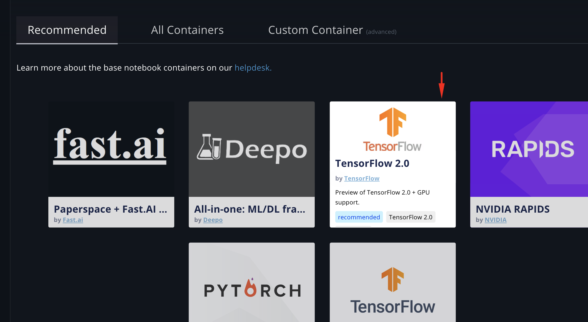
TensorFlow is one of the most popular frameworks used for deep learning projects and is approaching a major new release- TensorFlow 2.0. Luckily, we don't have to wait for the official release. A beta version is available to experiment on the official site and you can also use the preconfigured template on Paperspace Gradient. In this tutorial, we will go over a few of the new major features in TensorFlow 2.0 and how to utilize them in deep learning projects. These features are eager execution, tf.function decorator, and the new distribution interface. This tutorial assumes a familiarity with TensorFlow, the Keras API and generative models.
To demonstrate what we can do with TensorFlow 2.0, we will be implementing a GAN model. The GAN paper we will be implementing here is MSG-GAN: Multi-Scale Gradient GAN for Stable Image Synthesis. Here the generator produces multiple different resolution images and the discriminator decides on multiple resolutions given to it. By having the generator produce multiple resolution images, we ensure that the latent features throughout the network are relevant to output images.
Bring this project to life
Dataset Setup
The first step for training a network is to get the data pipeline started. Here we will be using the fashion MNIST dataset and use the established dataset API to create a TensorFlow dataset.
def mnist_dataset(batch_size):
    #fashion MNIST is a drop in replacement for MNIST that is harder to solve
    (train_images, _), (_, _) = tf.keras.datasets.fashion_mnist.load_data()
    train_images = train_images.reshape([-1, 28, 28, 1]).astype('float32')
    train_images = train_images/127.5  - 1
    dataset = tf.data.Dataset.from_tensor_slices(train_images)
    dataset = dataset.map(image_reshape)
    dataset = dataset.cache()
    dataset = dataset.shuffle(len(train_images))
    dataset = dataset.batch(batch_size, drop_remainder=True)
    dataset = dataset.prefetch(1)
    return dataset

#Function for reshaping images into the multiple resolutions we will use
def image_reshape(x):
    return [
        tf.image.resize(x, (7, 7)),
        tf.image.resize(x, (14, 14)),
        x
    ]
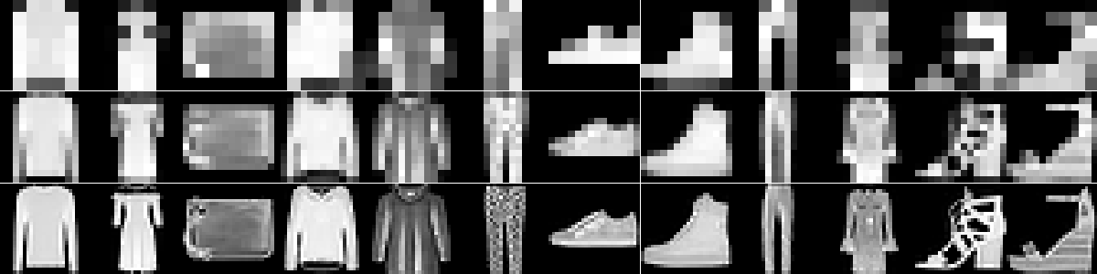
The eager execution implemented in TensorFlow 2.0 removes the need for initializing variables and creating sessions. With eager execution we can now use TensorFlow in a more pythonic way and debug as we go. This extends to the dataset api in TensorFlow and grants us the ability to interact with the data pipeline interactively through iteration.
# use matplotlib to plot a given tensor sample
def plot_sample(sample):
    import matplotlib.pyplot as plt
    import matplotlib.gridspec as gridspec
    num_samples = min(NUM_EXAMPLES, len(sample[0]))

    grid = gridspec.GridSpec(num_res, num_samples)
    grid.update(left=0, bottom=0, top=1, right=1, wspace=0.01, hspace=0.01)
    fig = plt.figure(figsize=[num_samples, 3])
    for x in range(3):
        images = sample[x].numpy() #this converts the tensor to a numpy array
        images = np.squeeze(images)
        for y in range(num_samples):
            ax = fig.add_subplot(grid[x, y])
            ax.set_axis_off()
            ax.imshow((images[y] + 1.0)/2, cmap='gray')
    plt.show()

# now lets plot a sample
dataset =  mnist_dataset(BATCH_SIZE)
for sample in dataset: # the dataset has to fit in memory with eager iteration
    plot_sample(sample)
Model Setup
We can move onto creating the generator and discriminator models, now that the dataset is made and verified. In 2.0, the Keras interface is the interface for all deep learning. That means the generator and discriminator are made like any other Keras model. Here we will make a standard generator model with a noise vector input and three output images, ordered from smallest to largest.
def generator_model():
    outputs = []

    z_in = tf.keras.Input(shape=(NOISE_DIM,))
    x = layers.Dense(7*7*256)(z_in)
    x = layers.BatchNormalization()(x)
    x = layers.LeakyReLU()(x)
    x = layers.Reshape((7, 7, 256))(x)

    for i in range(3):
        if i == 0:
            x = layers.Conv2DTranspose(128, (5, 5), strides=(1, 1),
                padding='same')(x)
            x = layers.BatchNormalization()(x)
            x = layers.LeakyReLU()(x)
        else:
            x = layers.Conv2DTranspose(128, (5, 5), strides=(2, 2),
                padding='same')(x)
            x = layers.BatchNormalization()(x)
            x = layers.LeakyReLU()(x)

        x = layers.Conv2D(128, (5, 5), strides=(1, 1), padding='same')(x)
        x = layers.BatchNormalization()(x)
        x = layers.LeakyReLU()(x)

        outputs.append(layers.Conv2DTranspose(1, (5, 5), strides=(1, 1),
            padding='same', activation='tanh')(x))

    model = tf.keras.Model(inputs=z_in, outputs=outputs)
    return model
Next we make the discriminator model.
def discriminator_model():
    # we have multiple inputs to make a real/fake decision from
    inputs = [
        tf.keras.Input(shape=(28, 28, 1)),
        tf.keras.Input(shape=(14, 14, 1)),
        tf.keras.Input(shape=(7, 7, 1))
    ]

    x = None
    for image_in in inputs:
        if x is None:
            # for the first input we don't have features to append to
            x = layers.Conv2D(64, (5, 5), strides=(2, 2),
                padding='same')(image_in)
            x = layers.LeakyReLU()(x)
            x = layers.Dropout(0.3)(x)
        else:
            # every additional input gets its own conv layer then appended
            y = layers.Conv2D(64, (5, 5), strides=(2, 2),
                padding='same')(image_in)
            y = layers.LeakyReLU()(y)
            y = layers.Dropout(0.3)(y)
            x = layers.concatenate([x, y])

        x = layers.Conv2D(128, (3, 3), strides=(1, 1), padding='same')(x)
        x = layers.LeakyReLU()(x)
        x = layers.Dropout(0.3)(x)

        x = layers.Conv2D(64, (5, 5), strides=(2, 2), padding='same')(x)
        x = layers.LeakyReLU()(x)
        x = layers.Dropout(0.3)(x)

    x = layers.Flatten()(x)
    out = layers.Dense(1)(x)
    inputs = inputs[::-1] # reorder the list to be smallest resolution first
    model = tf.keras.Model(inputs=inputs, outputs=out)
    return model

# create the models and optimizers for later functions
generator = generator_model()
discriminator = discriminator_model()
generator_optimizer = tf.keras.optimizers.Adam(1e-3)
discriminator_optimizer = tf.keras.optimizers.Adam(1e-3)
Training with tf.functions
With the generator and discriminator models created, the last step to get training is to build our training loop. We won't be using the Keras model fit method here to show how custom training loops work with tf.functions and distributed training. The tf.function decorator is one of the most interesting tools to come in TensorFlow 2.0. Tf.functions takes a given native python function and autographs it onto the TensorFlow execution graph.This gives a performance boost over using a traditional python function which would have to use a context switch and not take advantage of graph optimizations. There are number of caveats for getting this performance boost. The largest drop of performance comes from passing python objects as arguments and not TensorFlow classes. With this is mind, we can create our custom training loop and loss functions using the function decorator.
# this is the custom training loop
# if your dataset cant fit into memory, make a train_epoch tf.function
#    this avoids the dataset being iterarted eagarly which can fill up memory
def train(dataset, epochs):
     for epoch in range(epochs):
         for image_batch in dataset:
             gen_loss, dis_loss = train_step(image_batch)

# prediction of 0 = fake, 1 = real
@tf.function
def discriminator_loss(real_output, fake_output):
    real_loss = tf.nn.sigmoid_cross_entropy_with_logits(
        tf.ones_like(real_output), real_output)
    fake_loss = tf.nn.sigmoid_cross_entropy_with_logits(
        tf.zeros_like(fake_output), fake_output)
    return tf.nn.compute_average_loss(real_loss + fake_loss)

@tf.function
def generator_loss(fake_output):
    loss = tf.nn.sigmoid_cross_entropy_with_logits(
        tf.ones_like(fake_output), fake_output)
    return tf.nn.compute_average_loss(loss)

@tf.function
def train_step(images):
    noise = tf.random.normal([BATCH_SIZE, NOISE_DIM])

    #gradient tapes keep track of all calculations done in scope and create the
    #    gradients for these
    with tf.GradientTape() as gen_tape, tf.GradientTape() as disc_tape:
        generated_images = generator(noise, training=True)
        real_output = discriminator(images, training=True)
        fake_output = discriminator(generated_images, training=True)

        gen_loss = generator_loss(fake_output)
        dis_loss = discriminator_loss(real_output, fake_output)

    gradients_of_generator = gen_tape.gradient(gen_loss,
        generator.trainable_variables)
    gradients_of_discriminator = disc_tape.gradient(dis_loss,
        discriminator.trainable_variables)

    generator_optimizer.apply_gradients(zip(gradients_of_generator,
        generator.trainable_variables))
    discriminator_optimizer.apply_gradients(zip(gradients_of_discriminator,
        discriminator.trainable_variables))

    return gen_loss, dis_loss

# lets train
train(dataset, 300)
Distribution in 2.0
after our custom training loop is established its time to distribute it over multiple GPUs. In my opinion, the new strategy focused distribute API is the most exciting feature coming in 2.0. It is also the most experimental, not all distribution features are currently supported for every scenario. Using the distribute API is simple and requires a handful of modifications to the current code. to begin, we have to pick the strategy we want to use for distributed training. here we will use the MirroredStrategy. This strategy distributes work over available GPUs on a single machine. There are other strategies in the works, but this is currently the only supported strategy for custom training loops. Using strategies is simple; pick the strategy and then place code inside scope.
strategy = tf.distribute.MirroredStrategy()
with strategy.scope():
    # move all code we want to distribute in scope
    #    model creation, loss function, train functions
This interface is easy to use, and this is the only change that needs to be made when using the Keras fit method to train. We are using a a custom training loop, so we still have a few modifications to make. The dataset needs to be fixed first. Each training batch the dataset creates will be split up onto each GPU. A dataset with a batch size of 256 distributed over 4 GPUs will place batches of size 64 onto each GPU. We need to adjust the batch size of the dataset to use a global batch size, instead of the batch size we want per GPU. An experimental function also needs to be used to prepare the dataset for distribution.
NUM_GPUS = strategy.num_replicas_in_sync
dataset =  mnist_dataset(BATCH_SIZE * NUM_GPUS)
# we have to use this experimental method to make the dataset distributable
dataset = strategy.experimental_distribute_dataset(dataset)
The last step is to wrap the train step function with a distributed train function. Here we have to use another experimental function. This one requires us to give a non tf.function for it to distribute.
@tf.function
def distributed_train(images):
    gen_loss, dis_loss = strategy.experimental_run_v2(
        # remove the tf functions decorator for train_step
        train_step, args=(images,))
    # this reduces the return losses onto one device
    gen_loss = strategy.reduce(tf.distribute.ReduceOp.MEAN, gen_loss, axis=None)
    dis_loss = strategy.reduce(tf.distribute.ReduceOp.MEAN, dis_loss, axis=None)
    return gen_loss, dis_loss

# also change train() to use distributed_train instead of train_step
def train(dataset, epochs):
     for epoch in range(epochs):
         for image_batch in dataset:
             gen_loss, dis_loss = distributed_train(image_batch)
Now when I run with distribution I get the following numbers on 1070s.
- 1 GPU: average 200.26 ms/image
- 3 GPU: average 39.27 ms/image
We would expect 3x performance increase not a 5x increase, but hey, it is in beta.
Now we have used eager execution to inspect the data pipeline, used tf.functions for training, and used the new distribute api with a custom loss function.
Have fun exploring and working with TensorFlow 2.0. As a reminder, you can launch a GPU-enabled instance with TensorFlow 2.0 and all the necessary libraries, drivers (CUDA, cuDNN etc.) on Gradient in just a few clicks.