The Concept of Images In Image Processing

In order to properly grasp processes or concepts in Computer Vision or Image Processing in general, it is imperative to understand the very nature of digital imagery. In this article, we will be taking a look at what exactly constitutes images in a digital space so as to try to better understand and handle them.

Optical & Digital Perception

In an optical sense, when light bouncing off an object enters the human eye, signals are sent to the brain allowing us to perceive the object's shape and color. On the other hand, in a digital setting, a computer does not posses the ability to perceive shapes and colors rather it perceives an image as a collection of numbers in a spatial plane.

Properties of Digital Images

When talking about images in a digital context, three main properties often come to mind. They are, dimension, pixel and channel. In this section we will be looking at each one.

Dimension

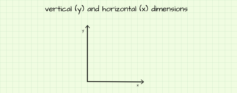
Also known as coordinate or axis, dimension represents a form of reference on a spatial plane (hence the term spatial dimension). Consider a plane sheet of paper propped up to stand on one of its edges such that it faces you.  Imagine we are on an arbitrary point on this plane, we would only be able to move vertically (up and down), horizontally (left and right) or some combination of the two (at an angle). Since all of your movement on this plane can be summarized using those two directions, in order to move around in any meaningful way we would need two reference lines, one horizontal called 'x' and the other vertical called 'y' as depicted below. To be more exact, the horizontal reference can be called dimension x and the vertical reference dimension y. Since these two dimensions are enough to describe any movement or figure on this sheet of paper we can say it is a 2-D (2-dimensional) representation.

Now imagine if that sheet of paper were to be just one of the six surfaces of a cube. All along we had been moving on this surface, the horizontal and vertical edge of the surface represent x and y respectively. So what if we would like to go into the center of the cube for instance, we would need another reference line which is perpendicular (90 degrees) to the surface which we are currently on. Let's call that reference line dimension z. All of a sudden we can now move anywhere inside this imaginary cube using all 3 dimensions so the cube is said to be a 3-D (3-dimensional) representation.

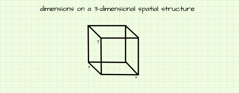
As we had mentioned earlier, all 3 reference lines that we have mentioned are called dimensions. If we have some kind of background in mathematics, we will find that the terms x, y and z are contextually accurate descriptions of axes/dimensions in a cartesian coordinate system (just another fancy name for a 3-D spatial structure). In a more geometrical sense, they would be called width, length and depth, in geography they would be longitude, latitude and altitude. However in image processing (using the Python Programming Language) they are termed dimension/axis 1, dimension/axis 0 and dimension/axis 2 respectively.

Dimensions & The Nomenclature of Position

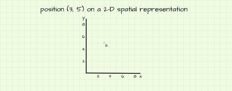
Any point on a spatial plane can be located by making reference to its position on all dimensions present. Consider a point k on a 2-D plane at a position (3, 5), this implies that the point is located 3 units from the origin on the x axis and 5 units from the origin on the y axis. For nomenclature purposes, points in a spatial structure are named (x-position, y-position) if they are present on a 2-D representation and (x-position, y-position, z-position) if they are on 3-D representations.

Pixels

Pixels are the numeric representations which make up a digital image. Their values could range from 0 (no intensity) to 1 (maximum intensity) when dealing with floating point values or from 0 (no intensity) to 255 (maximum intensity) when dealing with integer values. These pixels are put together to form a grid (rows and columns) in the dimensions mentioned in the previous section so as to form a 2-dimensional figure.

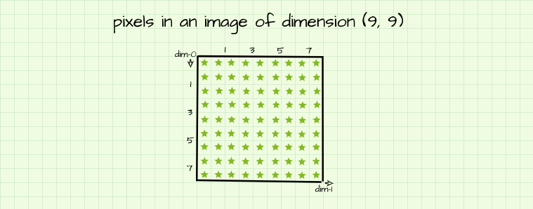
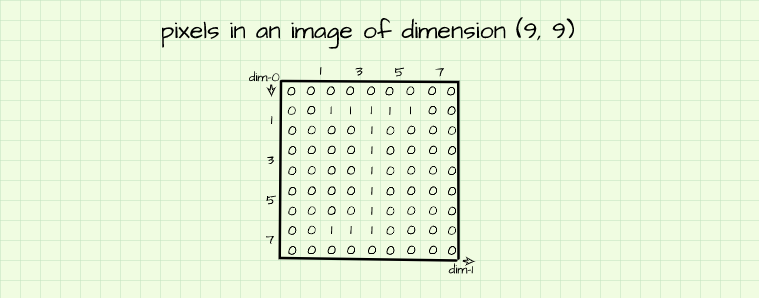
Consider the 2-D plane we used for illustration purposes in the last section. Imagine the axes are closed off to form a square as seen in the image above, it then essentially becomes a grid of 9 columns and 9 rows. When this grid is populated with pixels (depicted by the green stars just for convenience), it becomes an image of 9 rows by 9 columns which implies that there are 9 columns and 9 rows of pixels. In more succinct terms, it becomes a (9, 9) pixel image. To determine the number of total pixels present in this image, we simply multiply the number of units present in both dimension, in this case 9*9 = 81 pixels.

Pixels & The Nomenclature of Position

In the context of image processing using the Python Programming Language, there is going to be a slight modification to the 2-D plane we have been working with. Firstly, the origin of the plane is now to be situated at the top left corner instead of the bottom left corner. Secondly, axis-y is renamed to dimension-0/axis-0 and axis-x is renamed to dimension-1/axis-1. Lastly, numbering begins form 0, that is to say that the first measure after the origin is 0 instead of 1.

With all those changes implemented, we now have a standard Python array. The nomenclature of pixels in this image is basically the index of elements in the array. The pixel at the top right corner is located at an index [0, 8] since it is located on the first row (row 0) and the ninth column (column 8). In the same vane, pixels in the fifth row are indexed as [4] (row 4). Any pixel in an image can be located using array indexing in the form [row-number, column-number].

Creating Simple Images

In mathematics, there exists a mathematical formulation comprised of rows and columns, that formulation is called a matrix. Just like the sample (9, 9) image above, a matrix is populated with rows and columns of numeric types. In Python, a matrix can be created as an array using the NumPy library, it is therefore reasonable to say that a digital image is perceived as an array of pixels by the computer.

To prove this, we might as well just create a (9, 9) array of zeros and attempt to visualize it as shown below. As we can see, since all elements (pixels) in the array are 0 (no intensity), the array shows up as a blacked out image when visualized. Permit the usage of the 'cmap' parameter in the imshow() method for now, it will become clearer later.

#  import these dependencies
import numpy as np
import matplotlib.pyplot as plt

#  creating (9, 9) array of zeros
image = np.zeros((9, 9))

#  attempting to visualize array
plt.imshow(image, cmap='gray')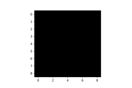

What happens when not all elements of the array are zero? Remember in the previous sections where it was mentioned that when dealing with integers, pixel values can range from 0 (no intensity) to 255 (maximum intensity). So theoretically, if we create an array filled with a range of progressively increasing integer values, we should obtain an image with pixels becoming progressively brighter. Let's see if this holds true in practice.

#  creating a 1-D array (vector) of elements ranging from 0 to 80
image = np.arange(81)
#  reshaping vector into 2-D array
image = image.reshape((9, 9))

#  attempting to visualize array
plt.imshow(image, cmap='gray')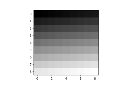

In the code block above, a '1-D array' (actually called a vector) with elements ranging form 0 to 80 is created (so a total of 81 elements). Next, the vector is reshaped into a (9, 9) array and then visualized. Evidently, since the pixels (elements) in the array increase from o to 80, pixel intensities increase progressively from dimmest to brightest, so in fact the pixel intensity theory does prove true.

image

array([[ 0,  1,  2,  3,  4,  5,  6,  7,  8],
       [ 9, 10, 11, 12, 13, 14, 15, 16, 17],
       [18, 19, 20, 21, 22, 23, 24, 25, 26],
       [27, 28, 29, 30, 31, 32, 33, 34, 35],
       [36, 37, 38, 39, 40, 41, 42, 43, 44],
       [45, 46, 47, 48, 49, 50, 51, 52, 53],
       [54, 55, 56, 57, 58, 59, 60, 61, 62],
       [63, 64, 65, 66, 67, 68, 69, 70, 71],
       [72, 73, 74, 75, 76, 77, 78, 79, 80]])

Variance & Relative Pixel Intensity

When dealing with pixels in an image, the intensity or brightness of each pixel is based on the overall nature of all pixels. In other words, there has to be a variation of pixel values for intensity to come into play. For instance, an array with all elements with a value of 100 will show up as a blacked out image (similar to the array of zeros) since the variance of its elements is o.

Furthermore, when dealing with integer pixel values, if all pixels are within the range of 0 and 10, pixel brightness will scale progressively between between those values, with 0 as the dimmest, 10 as maximum brightness and 5 as 5/11 of maximum brightness. However, if values are between 1 and 100, pixels with a value of 1 will appear dimmest, those with a value of 100 will appear brightest and those with a value of 10 will have a brightness of 1/10 of maximum.

Creating Meaningful Images

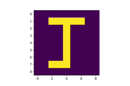
Its obviously becoming clearer that by putting together pixels of different intensities, one could produce a desired figure. Still utilizing our (9, 9) pixel 'canvas', let's attempt to produce the array shown below.

This array is made up of a bunch of zeros and ones with the ones seemingly highlighting the outline of the letter 'J'. Based on our knowledge of pixel intensities, we know that the 'zero' pixels have no intensity (no brightness) therefore they will appear black; we also know that the 'one' pixels will have a maximum intensity - maximum intensity in this case since 1 is the maximum value. It goes without saying that this array would produce a figure of the letter 'J' when visualized.

#  creating the array
image = np.zeros((9, 9))
image[1, 2:-2] = 1
image[1:-1, 4] = 1
image[-2, 2:4] = 1

plt.imshow(image)

So yes, putting together pixels with varying intensities will yield desired figures if done mindfully enough. The next question now would be if pixels can be put together to form more complex images like the image of a human face for instance? The answer to that question is an emphatic yes! Of course, we will need more than 81 pixels as a human face contains alot of details, but masterfully putting together pixels to form complex and realistic images is basically what generative models like Autoencoders, Generative Adversarial Networks and DALL-E are all about.

Basic Image Manipulation

With the realization that images are essentially arrays, comes the ability to manipulate them simply by interacting with their array representations. Any mathematical operation which applies to matrices also applies to digital images. In the same vane, any operation that applies to Python arrays, can apply to digital images, as well.

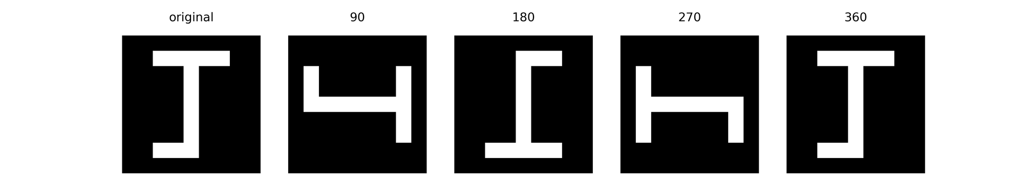
One very simple array operation which has a significant effect in the manipulation of images is array indexing and slicing. Simply by slicing arrays, one could rotate an image at right angles. The following code demonstrates this process.

def rotate(image_path, angle):
    """
    This function rotates images at right angles
    in a clockwise manner.
    """
    if angle % 90 != 0:
      print('can only rotate at right angles (90, 180, 270, 360)')
      pass
    else:
      #  reading image
      image = cv2.imread(image_path, cv2.IMREAD_GRAYSCALE)
      
      #  rotating image
      if angle == 90:
        image = np.transpose(image) #  transposing array
        image = image[:, ::-1] #  reversing columns
        plt.imshow(image, cmap='gray')
      elif angle == 180:
        image = image[::-1, :] #  reversing rows
        image = image[:, ::-1] #  reversing columns
        plt.imshow(image, cmap='gray')
      elif angle == 270:
        image = np.transpose(image) #  transposing array
        image = image[::-1, :] #  reversing rows
        plt.imshow(image, cmap='gray')
      else:
        image = image
        plt.imshow(image, cmap='gray')
    pass

Using the function above, image arrays can be manipulated in such a way that their pixels are rearranged to give rotated versions of the original image.

One could also explicitly change the value of pixels in an image by indexing and assigning them new values. For instance, let's assume we would like to generate a figure 'T' from our figure 'J'. Its a matter of simply canceling out the tail of the 'J' which is formed by pixels on row 7, columns 2 & 3. We can do this by indexing those pixels and assigning them a value of zero so they have no intensity.

#  indexing and assigning
image[7, 2:4] = 0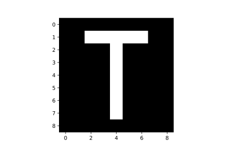

Channels

Channels are a property of images which determines their color. Casting our minds back to the 3-D spatial representation presented in the dimension section, to properly represent an image one needs to consider the z axis as well. Turns out that an image might not just be made up of a single array, it could be made up of a stack of arrays. Each array in the stack is called a channel.

Gray-scale images are made up of just one array, therefore they have just one channel like all the arrays we dealt with in the previous section. Colored images on the other hand are made up of 3 arrays laid on top of one another, therefore they have 3 channels (think of these channels as pieces of paper laid on top of one another).

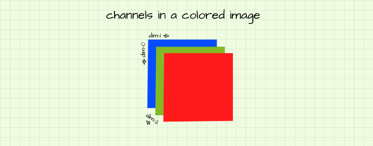
Channels In Colored Images

Each channel in a colored image represents an array of pixels which can only produce one of 3 colors, red, green, blue (RGB). In every colored image, these channels are always arranged the same with the first being red, the second being green and the third being blue.  

Based on the intensity of corresponding pixels across these 3 channels, any color could be formed. Lets put this to the test using the figure using our figure 'J'. We will attempt to create different variations of it, each variation will have a different color.

Red Colored J Atop A Black Canvas

As the topic states, we are attempting to create an image of a red figure 'J' with a black background. In order to generate a black background, we essentially need all pixels in the background to have no intensity, hence a pixel value of zero. Since we are trying to create a red figure, only the pixels outlining the figure in the red channel are 'switched on' allowing only the red color to shine through as shown above.

#  creating a 9x9 pixel image with 3 channels
image = np.zeros((9,9,3)).astype(np.uint8)

#  switching on pixels outlining the figure j in the red channel (channel 0)
image[1, 2:-2, 0] = 255
image[1:-1, 4, 0] = 255
image[-2, 2:4, 0] = 255

plt.imshow(image)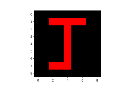

Green Colored J Atop A Black Canvas

Similar to the red figure produced above, to produce a green figure we need only to switch on its outlining pixels in the green channel.

#  creating a 9x9 pixel image with 3 channels
image = np.zeros((9,9,3)).astype(np.uint8)

#  switching on pixels outlining the figure j in the green channel (channel 1)
image[1, 2:-2, 1] = 255
image[1:-1, 4, 1] = 255
image[-2, 2:4, 1] = 255

plt.imshow(image)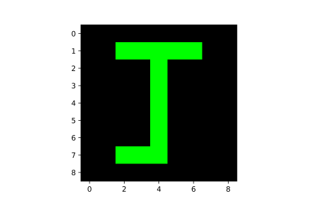

Blue Colored J Atop A Black Canvas

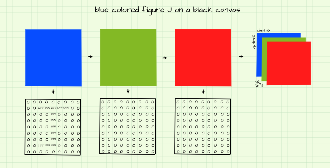
Likewise, to produce a blue figure on a black background, only the outlining pixels in the blue channel are switched on as shown above.

#  creating a 9x9 pixel image with 3 channels
image = np.zeros((9,9,3)).astype(np.uint8)

#  switching on pixels outlining the figure j in the blue channel (channel 2)
image[1, 2:-2, 2] = 255
image[1:-1, 4, 2] = 255
image[-2, 2:4, 2] = 255

plt.imshow(image)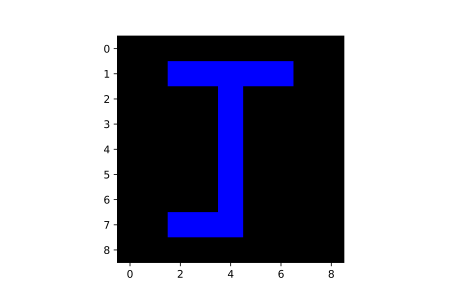

Teal Colored J Atop A Burgundy Canvas

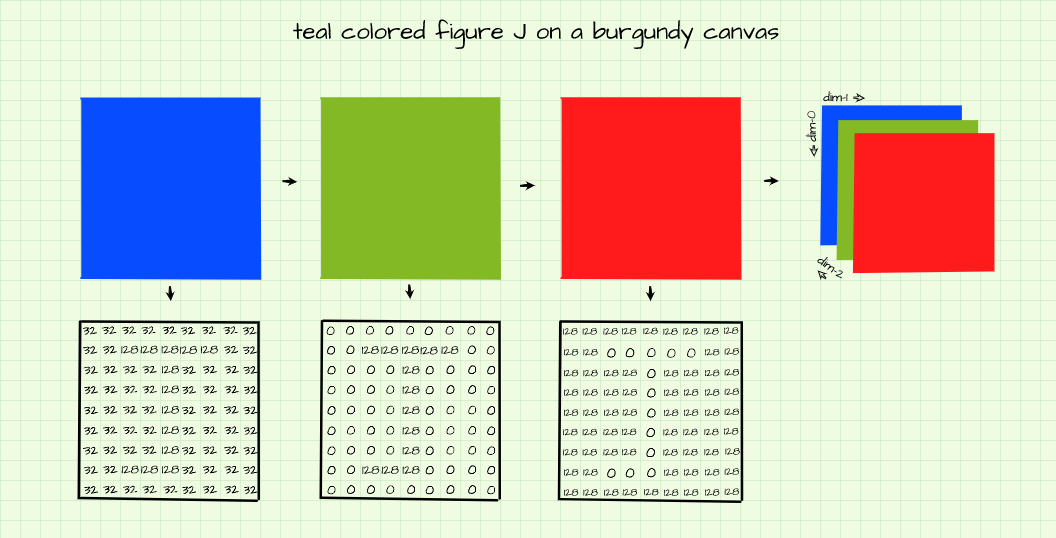
Now for something more complex. The goal is to produce an image of a teal colored figure 'J' with a burgundy background. In order to produce a burgundy background, the burgundy RGB values (128, 0, 32) need to be replicated across corresponding channels for pixels which make up the background.

In the same vane, to produce a teal colored figure 'J', the teal RGB values (0, 128, 128) need to be assigned to outline pixels in corresponding channels as shown in the image above and replicated in the code block below.

#  creating array
image = np.zeros((9,9,3)).astype(np.uint8)

#  assigning background color in each channel
image[:,:,0] = 128
image[:,:,1] = 0
image[:,:,2] = 32

#  outlining figure j in each channel
image[1, 2:-2, 0] = 0
image[1, 2:-2, 1] = 128
image[1, 2:-2, 2] = 128

image[1:-1, 4, 0] = 0
image[1:-1, 4, 1] = 128
image[1:-1, 4, 2] = 128

image[-2, 2:4, 0] = 0
image[-2, 2:4, 1] = 128
image[-2, 2:4, 2] = 128

plt.imshow(image)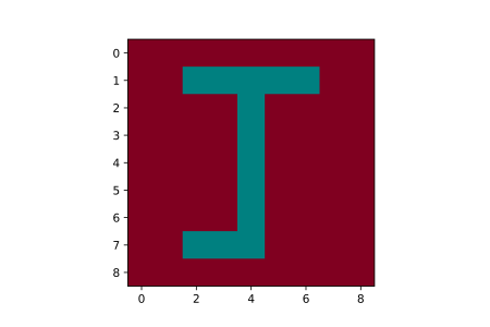

Color To Grayscale

Since the only thing which distinguishes color and grayscale images in a digital context is the number of channels, theoretically if we can find a way to compress all 3 channels in a colored image into just one channel we could convert colored images into grayscale images. The theory works.

There are several techniques to do this, however, the simplest way is to simply take the average of corresponding pixels across channels.

#  computing the average value of pixels across channels
image = image.mean(axis=2)

Grayscale Images In Matplotlib

As stated previously, grayscale (black and white) images have just one channel, similar to the single arrays used in previous sections. However, when visualizing these single arrays we had to utilize the 'cmap' parameter in Matplotlib. The reason for doing this is because Matplotlib does not implicitly recognize single channel arrays as image data so they do not get visualized as grayscale rather they get visualized as color-maps.

However, in order to produce a grayscale version of the above image (which was archived by setting cmap='gray'), we need to create a 3 channeled array, set background pixels to zero and switch on outline pixels on each channel to full intensity (255) as that will produce a black background and a white (255, 255, 255) figure.

#  creating array
image = np.zeros((9,9,3))

#  setting outline 
image[1, 2:-2, :] = 255
image[1:-1, 4, :] = 255
image[-2, 2:4, :] = 255

plt.imshow(image)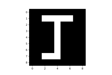

Final Remarks

In this article we have been able to develop an intuition about the essential elements that make up a digital image. We went from discussing about dimensions, which serve as reference points in a spatial structure, to pixels, numeric types which form images using their brightness, and finally channels, which help to form color by combining different intensities of red, blue and green.