The advent of diffusion models for image synthesis has been taking the internet by storm as of late. There is good reason for this. Following the release of CompVis's "High-Resolution Image Synthesis with Latent Diffusion Models" earlier this year, it has become evident that diffusion models are not only extremely capable at generating high quality, accurate images to a given prompt, but that this process is also far less computationally expensive than many competing frameworks.

In this blogpost, we will examine the basics of diffusion modeling, before exploring the corresponding advancements enabled by the new framework, Stable Diffusion. Next, we examine the advantages and disadvantages of using the model in its current state. We then conclude by jumping into a short coding demo that shows how we can run Stable Diffusion for free on a Gradient Notebook. By the end of this blog post, readers will be able to generate their own novel artwork/images using the model while building an understanding of how Stable Diffusion modeling operates under the hood.  

Introduction to Diffusion Models

At their core, Diffusion Models are generative models. In computer vision tasks specifically, they work first by successively adding gaussian noise to training image data. Once the original data is fully noised, the model learns how to completely reverse the noising process, called denoising. This denoising process aims to iteratively recreate the coarse to fine features of the original image. Then, once training has completed, we can use the Diffusion Model to generate new image data by simply passing randomly sampled noise through the learned denoising process.

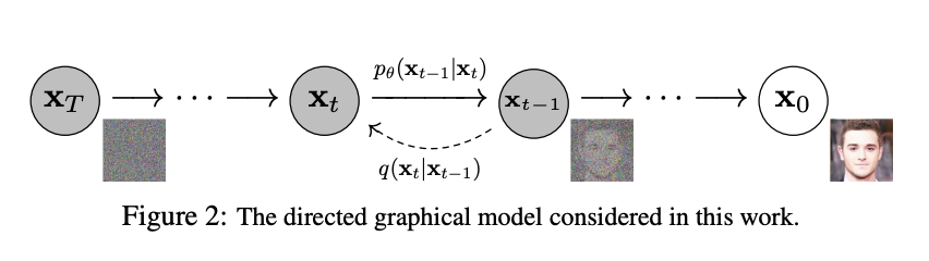
It achieves this by mapping the image's latent space using a fixed Markov Chain. The chain gradually adds the noise to the data in order to make the data approximate a posterior function, $ q(X1:T|X0) $. It assumes that $X0,...,XT$ are the images latent variables with the same dimensionality as $X0$. By the end of the sequence, the image data is transformed to the point it resembles pure Gaussian noise. Thus, the diffusion model must learn to reverse this process to get the desired generated image. The Diffusion Model is therefore trained by finding the reverse Markov transitions that maximize the likelihood of the training data.

Stable Diffusion

Stable Diffusion, the follow up to the same teams previous work on Latent Diffusion Models, improved significantly on predecessors both in image quality and scope of capability. It achieved this through a more robust training dataset and meaningful changes to the design structure.

This model uses a frozen CLIP ViT-L/14 text encoder to condition the model on text prompts. The dataset used for training is the laion2B-en, which consists of 2.32 billion image-text pairs in the English language. After training, with its 860M UNet and 123M text encoder, the model is relatively lightweight and can be run on a GPU with at least 10GB VRAM. It can be further optimized to run on GPUs with ~8 GB of VRAM, as well, by lowering the precision of the number format to half-precision (FP16).

In practice, these changes allow Stable Diffusion to excel in a number of computer vision tasks, including:

• Semantic synthesis - generating images solely via conditioning from text prompts
• Inpainting - filling in missing parts of images precisely, using deep learning to predict the features of the missing part of the image
• Super-resolution - a class of techniques that enhance (increase) the resolution of an imaging system

What's new with Stable Diffusion?

Better scaling

One of the key ways Stable Diffusion differs from past methodologies for diffusion modeling is the ability to scale much more easily. Previous, related works, such as GAN based methods or pure transformer approaches, require heavy spatial downsampling in the latent space in order to reduce the dimensionality of the data. Because Diffusion Models already offer such excellent inductive biases for spatial data, the effect of downsampling the latent space being removed is inconsequential to our final output quality.

In practice, this allows for two extensions of the models capabilities: to work on a compression level which provides more faithful and detailed reconstructions than previous work, and to work efficiently for high resolution synthesis of large images.

Lower cost to run training and inference

Stable Diffusion is comparatively computationally inexpensive to run when compared to other SOTA competitor frameworks. The authors were able to show competitive performance levels for inpainting, unconditional image synthesis, and stochastic super-resolution generation tasks with significantly lower cost to run when compared to other methods. They were also able to significantly decrease the inference cost when compared to pixel-based diffusion approaches.

Flexibility

Many previous works on this model framework required a delicate weighting of the reconstruction and generation abilities of the model, as they learned the encoder/decoder architecture and a score based prior simultaneously. In contrast to previous works, stable diffusion does not require this delicate weighting of the reconstruction and generative abilities, which allows for more faithful reconstructions of images with relatively little regularization of the latent space.

High resolution image generation for densely conditioned tasks

When conducting densely conditioned tasks with the model, such as super-resolution, inpainting, and semantic synthesis, the stable diffusion model is able to generate megapixel images (around 10242 pixels in size). This capability is enabled when the model is applied in a convolutional fashion.

Stable Diffusion: uses of the model & comparison with competitor models

Now that we have an understanding of how diffusion works and why Stable Diffusion is so powerful, it is important to understand when this model should be used and when not to. Specifically, the model was designed for research purposes in general. Some potential research cases include:

• Safe deployment of models which have the potential to generate harmful content
• Probing and understanding the limitations and biases of generative models
• Generation of artworks and use in design and other artistic processes
• Applications in educational or creative tools
• Research on generative models [source]

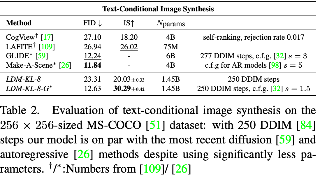
When acting on these tasks, Stable Diffusion is considered to be SOTA in terms of synthesis capability. As we can see from the table above, when performing a text-conditional image synthesis task, the predecessor to Stable Diffusion (Latent Diffusion) was able to achieve comparable FID scores to two of the top image synthesis model frameworks, GLIDE and Make-A-Scene. Furthermore, the LDM-KL-8-G was able to achieve the highest Inception Score (IS) of all the tested models. Based on this data, we can infer that Stable Diffusion is an extremely powerful image synthesis tool with accurate recreations. These findings are also reflected by the model when performing other tasks, indicating the model's general robustness.

Stable Diffusion: Problems with the model

While Stable Diffusion has state of the art capabilities, there are still situations where it will be inferior to others on certain tasks. Like many image generation frameworks, Stable Diffusion has built in limitations created by a number of factors, including the natural limitations of an image dataset during training, bias introduced by the developers on these images, and blockers built into the model to prevent misuse. Let's break down each of these.

Training set limitations

The training data used for an image generation framework will always have a significant impact on the scope of its abilities. Even when working with massive data, like the LAION 2B(en) dataset used for training Stable Diffusion, it is possible to confound the model by referencing unseen image types with the input prompt. Features that are not included in the original training step will be impossible to recreate, as the model has no understanding of these features.

This is most clearly exemplified by human figures and faces. The model was largely not trained with a focus on refining these features in the generated outputs. Be aware of these limitations if that is your intended use for the model.

Bias introduced by researchers

The researchers behind Stable Diffusion recognized the effect on social bias inherent in such a task. Primarily, Stable Diffusion v1 was trained on subsets of the LAION-2B(en) dataset. This data is nearly entirely in the English language. They posit that texts and images from cultures and communities that do not speak English would be largely unaccounted for. This choice to focus on these English language data enables a more robust connection between the English language prompts and the outputs, but simultaneously affects outputs by forcing white and western cultural influences to be dominant traits in the outputted images. On a similar note, the ability to use non-English language input prompts is inhibited by this training paradigm.

Built in blockers towards sexual, violent, and malicious image content

The authors of the model architecture have set and defined a list of contexts for using Stable Diffusion that would be characterized as abusive. This includes, but is not limited to:

• Generating demeaning, dehumanizing, or otherwise harmful representations of people or their environments, cultures, religions, etc
• Intentionally promoting or propagating discriminatory content or harmful stereotypes
• Impersonating individuals without their consent
• Sexual content without consent of the people who might see it
• Mis- and disinformation
• Representations of egregious violence and gore
• Sharing of copyrighted or licensed material in violation of its terms of use
• Sharing content that is an alteration of copyrighted or licensed material in violation of its terms of use - [source]

Code Demo

Now that we understand the basics of diffusion, the capabilities of the Stable Diffusion model, and the limitations we must operate under when using the model, we can jump into the coding demo to use Stable Diffusion to generate our own new images. Click on the link below to open a Notebook with a free GPU to test this code out.

Set up

First, we will do some necessary installs. Notably, we will be using diffusers to source the dataset and pipeline our training, and flax to perform CLIP reranking of our images by accuracy to the prompt.

!pip install --upgrade diffusers transformers scipy ftfy
!pip install flax==0.5.0 --no-deps
!pip install ipywidgets msgpack rich 

Next, you will need to gain access to the pretrained models for Stable Diffusion. In order to do that, you must login to Huggingface and create a token. Once that's done, go to the Stable Diffusion model page to acknowledge and accept their terms of use for the model that we discussed earlier. Once you have done that, paste your token into the notebook where it says <your_huggingface_token>. Then, run the cell. This will also create an outputs directory to save our generated samples in later on.

!python login.py --token <your_huggingface_token>
!mkdir outputs

Inference

Now that we have completed set up, we can get started generating our images. In the following example, we show how to run the image generation process on a machine with less than 10 GB of VRAM.

# Low cost image generation - FP16

import torch
from torch import autocast
from diffusers import StableDiffusionPipeline

model_id = "CompVis/stable-diffusion-v1-4"
device = "cuda"
pipe = StableDiffusionPipeline.from_pretrained(model_id, torch_dtype=torch.float16, revision="fp16", use_auth_token=True)
pipe = pipe.to(device)

sample_num = 10
lst = []
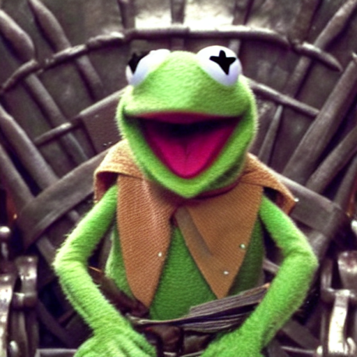
prompt = "Kermit the Frog on the Iron Throne"
for i in range(sample_num):
    with autocast("cuda"):
        lst.append(pipe(prompt, guidance_scale=7.5)["sample"][0])

    
for i in range(sample_num):
    lst[i].save(f'outputs/gen-image-{i}.png')

Let's walk through this. First, we import or packages and define the model_id and device variables. These will guide our StableDiffusionPipeline to download the appropriate model from HuggingFace Hub, set the model to work on half-precision data, and let it know it must use our authorization token to access the model files. We then use the .to method to move the pipeline to run on our GPU.

Next, we define sample_num and lst. The former represents the number of images we would like to generate, and the latter will hold our image data for ranking later. Then, the prompt can be changed to whatever the user deems appropriate.  Finally, we are ready to generate our images by looping for the range of sample_num, and generating a new image from the prompt to append to lst on each step. These are then finally saved to the outputs/ folder for examination later. Here is a sample from when we ran the same code as above:

CLIP ranking of the images

While it is pretty simple to take a qualitative assessment of the sample images, we can leverage the powerful CLIP model here to quantitively assess and rank the images based on their final image encodings proximity to the original input prompt encoding. This code is adapted from Boris Dayma's DALL-E Mini.

from transformers import CLIPProcessor, FlaxCLIPModel
import jax
import jax.numpy as jnp
from flax.jax_utils import replicate
from functools import partial


# CLIP model
CLIP_REPO = "openai/clip-vit-base-patch32"
CLIP_COMMIT_ID = None

# Load CLIP
clip, clip_params = FlaxCLIPModel.from_pretrained(
    CLIP_REPO, revision=CLIP_COMMIT_ID, dtype=jnp.float16, _do_init=False
)
clip_processor = CLIPProcessor.from_pretrained(CLIP_REPO, revision=CLIP_COMMIT_ID)
clip_params = replicate(clip_params)

# score images
@partial(jax.pmap, axis_name="batch")
def p_clip(inputs, params):
    logits = clip(params=params, **inputs).logits_per_image
    return logits

First, we load in the CLIP model and processor, replicate the params, and define our p_clip scoring function.

from flax.training.common_utils import shard
import numpy as np
# get clip scores
clip_inputs = clip_processor(
    text=prompt * jax.device_count(),
    images=lst,
    return_tensors="np",
    padding="max_length",
    max_length=77,
    truncation=True,
).data
logits = p_clip(shard(clip_inputs), clip_params)

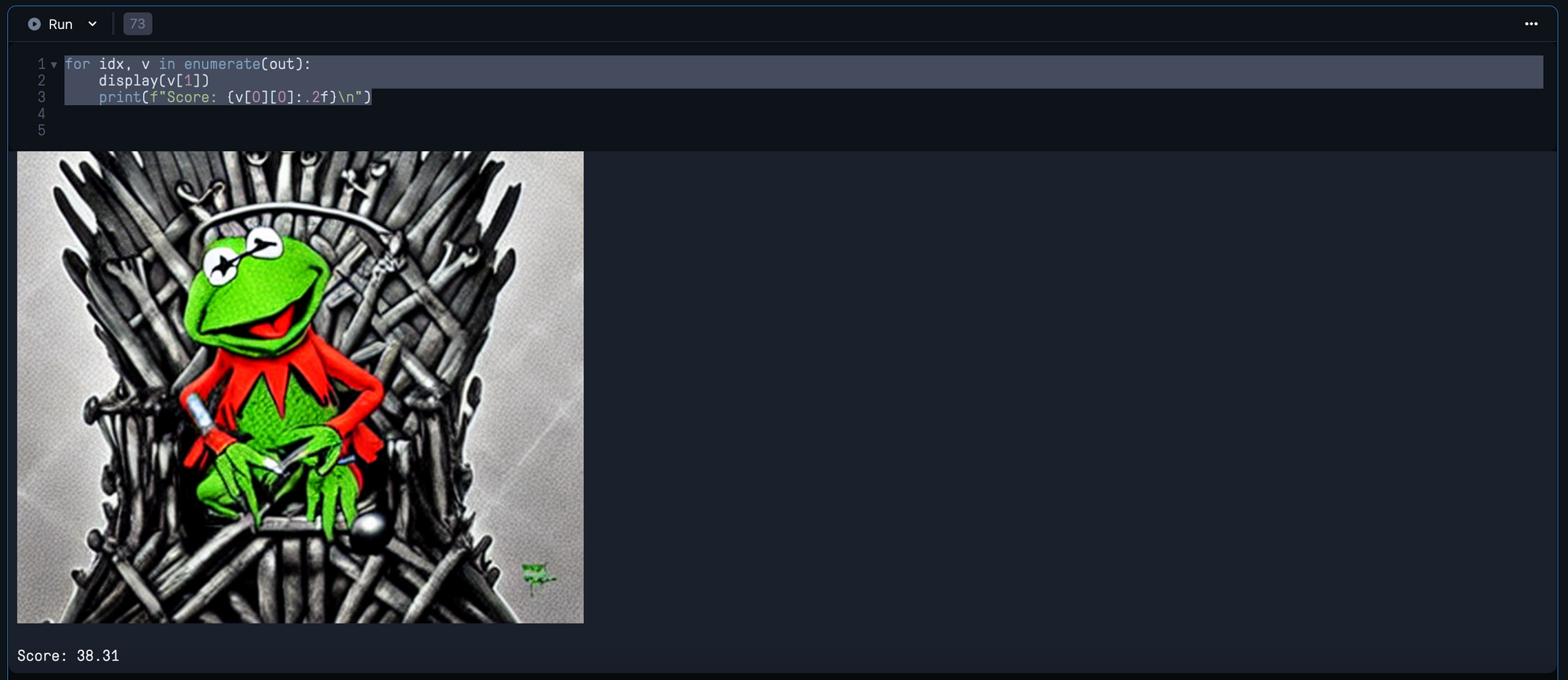
out = list(reversed(sorted(zip(logits[0], lst))))

for idx, v in enumerate(out):
    display(v[1])
    print(f"Score: {v[0][0]:.2f}\n")

We then get CLIP scores for each of the images with the CLIP processor with the clip_processor. We can then zip and sort these with our original list of images to create a merged list of the images ranked by their score.

With CLIP ranking, we can use both our own qualitative assessments in conjunction with a more objective quantitative scoring of the image generation. By itself, CLIP will do a suitable job of finding the best image given a prompt, but it is when combined with a human agent that we can find the best generated image.

Closing thoughts

In conclusion, Stable Diffusion is a powerful and easy to use image synthesis framework. We walked through how diffusion works, what is new and powerful with Stable Diffusion models, and then detailed the strengths and weaknesses of the framework. Afterwords, we showed how to perform text-conditional image synthesis with the technique on a Gradient Notebook.

Play around with these notebooks to see what cool and unique artwork you can generate, for free, today!