Top 4 Techniques for Handling Missing Values in Machine Learning

Data is increasingly becoming a premium for everyone on the internet, and turning information into data is becoming ever increasingly critical for all sorts of business problems. While data is obtained occasionally from websites such as Kaggle.com and various sources by web scraping on websites, this data frequently contains missing data. However, can that data be used to construct machine-learning algorithms? 

The answer is NO. This is because the data is raw and unprocessed. So, data preprocessing is required here before building the model. Data preprocessing includes handling missing data and converting categorical data to numerical data using techniques like One-hot encoding.

This article will explore different types of missing data and investigate the reasons behind missing values and their implications on data analysis. Furthermore, we will discuss different techniques to address missing values.

So, let's explore how to handle them efficiently in machine learning.

What are missing values? Why do they exist?

Data that is not present in a dataset.

Missing values are missing information in a dataset. It is like the missing piece in a zigzag puzzle, leaving gaps in the landscape. In the same way, missing values in data result in incomplete information. This makes it challenging to understand or accurately analyze the data and, as a result, results in inaccurate results or may lead to overfitting. 

In datasets, these missing entries might appear as the letter "0", "NA", "NaN", "NULL", "Not Applicable", or "None”. 

But you can handle these missing values easily with the techniques explained below. The next question is, why are missing values in the data?

Missing values can occur due to various factors like

• Failure to record data,
• Data corruption,
• Lack of information as some people have hesitation in sharing the information,
• System or equipment failures,
• Intentional omission.

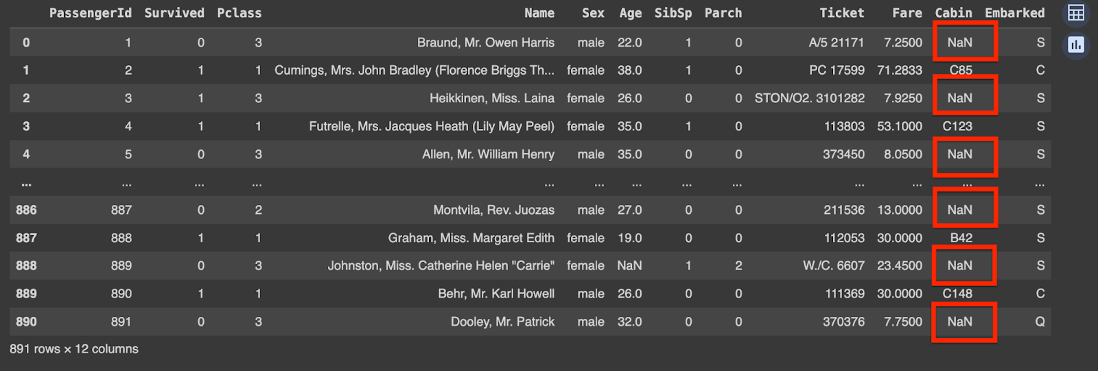
You can see that there are missing values in the ‘Cabin’ column. Missing values are represented by ‘NaN’ here.

Different Types of Missing Data

1) MCAR – "completely randomly missing" 

This occurs when all variables and observations are missing with equal probability. For instance, a survey's responses are missing due to technical glitches such as a computer malfunction. Removing MCAR data is safe as it does not introduce bias into the analysis.

2) MAR – "I missed it by accident" 

In MAR, the probability of missing value depends on the value of the variable or other variables in the data set. This means that not all variables and observations have the same probability of being missing. For instance, if data scientists don't upgrade their skills frequently and skip certain questions because they lack knowledge of cutting-edge algorithms and technologies. In this case, the missing data relates to how often data scientists continue their training. 

3) MNAR – "I didn’t lose it by accident"

MNAR is considered the most difficult scenario among the three types of missing data. In this case, the reasons for missing data may be unknown. An example of MNAR is a survey of married couples. Couples with bad relationships may not want to answer certain questions because they are embarrassed to do so.

Techniques to Handle Missing Values

We will discuss three primary methods: 

1. Deleting Rows with Missing Values

The simplest and easiest approach to handle missing values is to remove the rows or columns containing missing values in the dataset. The question that comes to mind is whether we will lose information if we delete the data. The answer is YES. Removing too many observations can reduce the statistical power of the analysis and lead to biased results. 

When to use this technique:

• You can delete the entire column if a particular column is missing many values. 
• If you have a huge dataset. Then, removing 2-3 rows/columns won't make much difference. 
• The output results do not depend on deleted data.
• Low variability in data or repetitive values.
• When datasets have highly skewed distributions, removing rows with missing values will be the best choice compared to imputation.

Note: This approach should be used in the above scenarios only and is not recommended much.

Let's take a look at an example of deletion using Python:

data.dropna(inplace=True)dropna(how = ‘all’) #the rows where all the column values are missing.

2. Imputation Techniques

Substituting reasonable estimates or guesses for missing values. 

Imputation methods are particularly useful when: 

• The percentage of missing data is low.
• Deleting rows would result in a significant loss of information.

Let's explore some of the commonly used imputation methods:

Mean, Median, or Mode Imputation

This approach replaces the missing values with the mean, median, or mode of the non-missing values in the respective variable.

• Mean: It is the average value.

Mean = (Sum of all values) / Number of values= 354/6

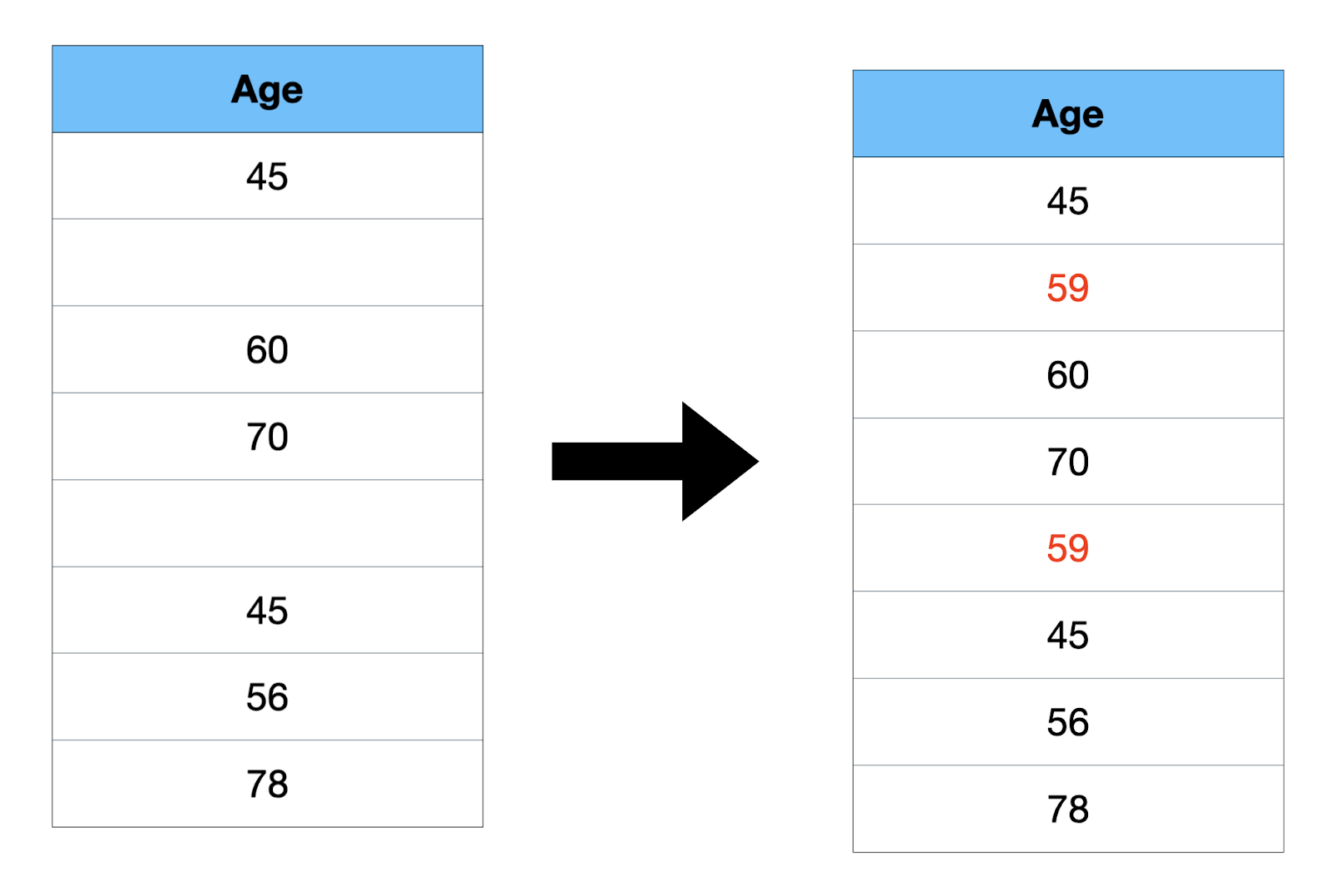
• Median: It is the midpoint value.

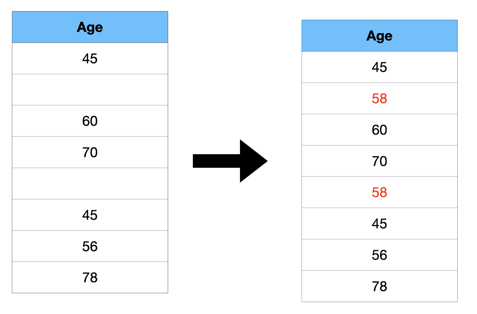
Arrange all the numbers in ascending order: 45, 45, 56, 60, 70, 78. The median is calculated as (56 + 60) / 2 = 116 / 2 = 58. If the number of data points is even, the median is the average of the two middle numbers.

• Mode: It is the most common value in the data.

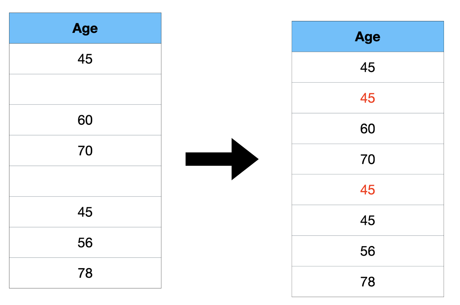
Here, 45 is repeated twice, so the mode value is 45.

Using Python, we can impute missing values with the mean or median as follows:

# Importing the necessary libraries
import pandas as pd
from sklearn.impute import SimpleImputer

# Loading the dataset
data = pd.read_csv('dataset.csv')

# Imputing missing values with mean
imputer = SimpleImputer(strategy='mean')
data['column_name'] = imputer.fit_transform(data[['column_name']])```

In the above example, the SimpleImputer class is used from the Scikit-learn library to impute missing values with the mean. The strategy parameter can be set to 'mean', 'median', or 'most_frequent'. The fit_transform() function replaces missing values with imputed ones.

3. Forward Fill and Backward Fill

Forward fill (ffill) and backward fill (bfill) are imputation techniques that use the values from previous or next observations to fill in the missing values. 

Forward Fill

Forward fill replaces missing values with the previous non-missing value. For instance, if there are missing values in the stock dataset for a weekend, you can forward fill the missing values with the last observed value from Friday.

Let’s understand with an example.

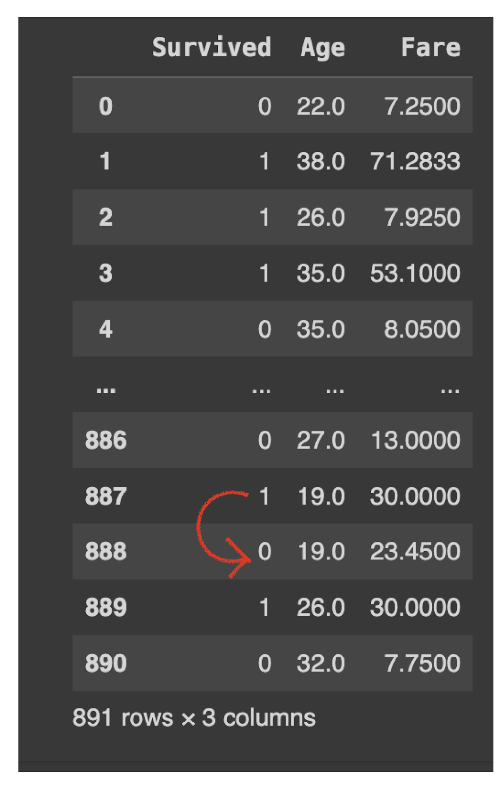
In this row, 888 had a missing value for the ‘Age’ column. So after running data['column_name'].fillna(method='ffill', inplace=True). So, the value ‘19’(previous value) is copied in place of the missing cell below.

Backward Fill

Backward fill replaces missing values with the next available non-missing value. For instance, if there are missing values in a temperature dataset, the next recorded value will be suitable and is considered the better estimate for the missing period, especially if the temperature is stable or changes predictably.

Let’s understand with an example.

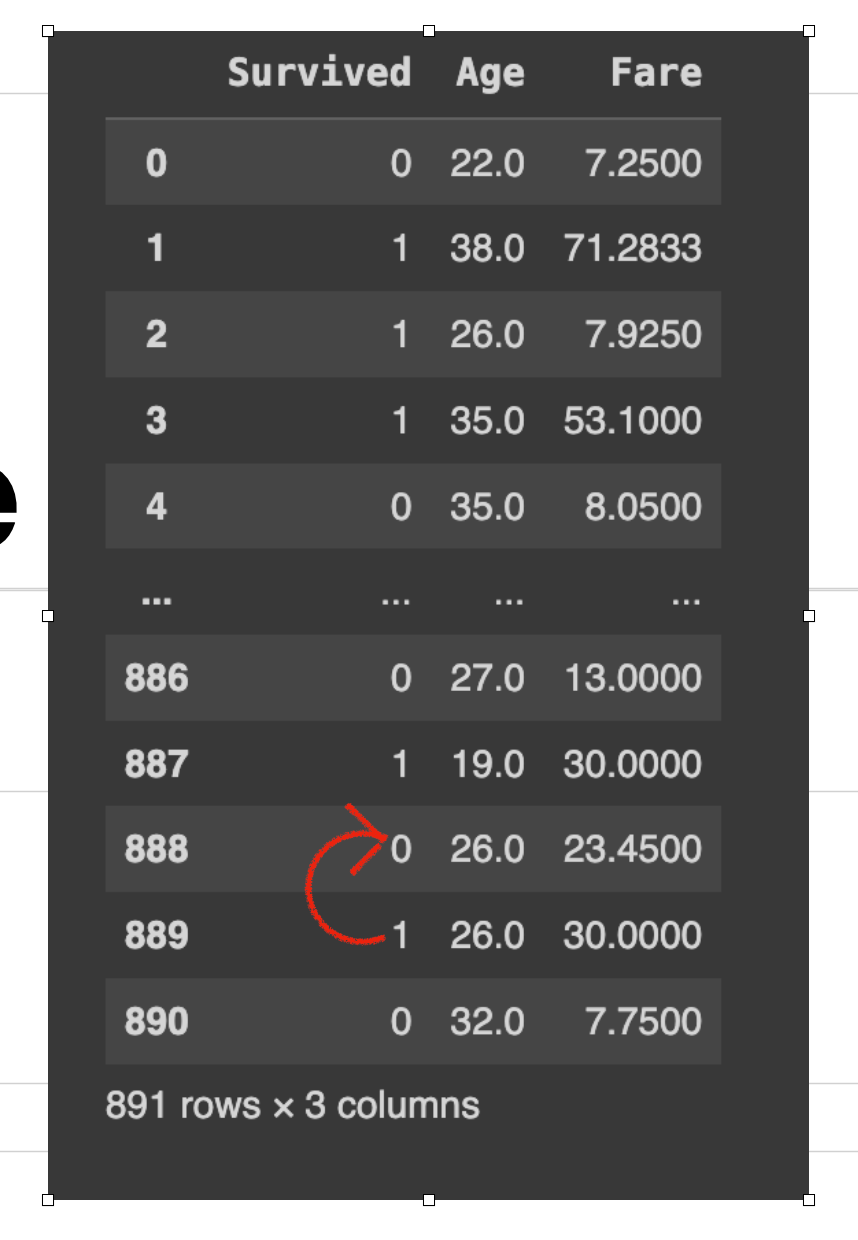
In this row, 888 had a missing value for the ‘Age’ column. So after running data['column_name'].fillna(method='bfill', inplace=True). So, the value ‘26’(next value) is copied in place of the missing cell above.

Using Pandas, we can perform forward fill and backward fill as follows:

4. Replacing with Arbitrary Value

Another approach to impute missing values is to replace them with an arbitrary value. Missing values (NA) are replaced with a pre-selected arbitrary number. The choice of this number can vary; common examples include 999, 9999, or -1. Choose the value carefully. This can be done by data['column_name'].fillna(-999, inplace=True)

we use the fillna() function to replace missing values in the 'column_name' column with the arbitrary value -999.

First, Understanding the root cause of missing values is crucial for selecting appropriate techniques to handle them effectively. Secondly, the method for handling missing values depends on the 

Demo

This project is very easy to set up. Just load 'titanic.csv' into Paperspace. Just click 'start machine' and let's get started. Let's take a look at an example using Python:

# Importing the necessary libraries

import pandas as pd
import numpy as np

# Loading the dataset
# Here, we're reading a CSV file named 'titanic.csv' and selecting only the 

'Age', 'Fare', and 'Survived' columns.
df = pd.read_csv("titanic.csv", usecols=['Age','Fare','Survived'])

# Displaying the DataFrame
df

# Checking for missing values in each column
df.isnull().sum()

# Filling missing 'Age' values with the mean age
# This line replaces all NaN (Not a Number) values in the 'Age' column with the mean (average) age.

df['Age'].fillna(df['Age'].mean(), inplace = True)

# Filling missing 'Age' values with the median age
# This line is redundant after the previous fillna, as there should be no NaN values left to replace.
# If there were, it would replace them with the median age.

df['Age'].fillna(df['Age'].median(), inplace = True)

# Filling missing 'Age' values with the mode
# This line is also redundant after the first fillna. It would replace NaN values with the mode (most frequent value).

df['Age'].fillna(df['Age'].mode(), inplace = True)

# Forward filling of missing values
# This replaces NaN values in the DataFrame with the previous non-null value along the column.
# If the first value is NaN, it remains NaN.

df.ffill(inplace=True)

# Backward filling of missing values
# This replaces NaN values with the next non-null value along the column.
# If the last value is NaN, it remains NaN.

df.bfill(inplace=True)

We have used the dataset 'titanic.csv'. This dataset is available on Kaggle. We focus on specific columns ('Age', 'Fare', 'Survived'). You can check for missing values in the dataset using isnull().sum(). This step is optional. Subsequently, it demonstrates various methods to impute these missing values in the 'Age' column: first by replacing them with the column's mean, then the median and mode. Then forward filling (ffill) and backward filling (bfill) methods were applied, propagating next or previous valid values to fill gaps. Finally, the remaining missing values are replaced with an arbitrary value (-999).To apply these changes directly to the DataFrame, inplace=True is used.

Note: Each subsequent method is redundant as the previous line already replaces all missing values. So choose one method out of these, checking the type of data and also checking how much data is missing.

Conclusion

Remember, missing values are not an obstacle; they are an opportunity to implement robust and innovative techniques to enhance the quality of your machine-learning models. So, embrace the challenge of missing values and employ the right techniques to unlock the true potential of your data.

We discussed the importance of understanding the reasons behind missing values and distinguishing between different types of missing data. We explored techniques such as deleting rows with missing values, imputation methods like mean/median/mode imputation, forward fill, backward fill, replacing arbitrary values, and using predictive models.