In this tutorial, we will explore the distilled version of Stable Diffusion (SD) through an in-depth guide, this tutorial also includes the use of Gradio to bring the model to life. Our journey begins with building comprehension of the knowledge distilled version of stable diffusion and its significance. To better understand the concept of Knowledge Distillation (KD), we've extensively covered it in a previous blog post. You can refer to the link provided for a detailed understanding of KD.
Furthermore, we will try to breakdown the model architecture as explained in the associated research paper. We will use this to help us run the project's included code demo, allowing us to gain a hands-on experience with the model using the free GPUs offered by Paperspace. We can easily run the model using on the platform with the provided Run on Paperspace link at the top of this page. Use the provided notebook to follow along and recreate the work shown in this article.
Engaging with the code demo will provide a practical grasp of utilizing the model, contributing to a well-rounded learning experience. We also encourage you to check out our previous blog posts on Stable Diffusion if interested in learning more about underlying base model.
Introduction
SD models are one of the most famous open-source models in general, though most importantly for their capabilities in text to image generations. SD has shown exceptional capabilities and has been a backbone in several text to image generation applications. SD models are latent diffusion models, the diffusion operations in these models are carried in a semantically compressed space. Within a SD model, a U-Net performs an iterative sampling to gradually remove noise from a randomly generated latent code. This process is supported by both a text encoder and an image decoder, working collaboratively to generate images that align with provided text descriptions or the prompts. However, this process becomes computationally expensive and often hinders in its usage. To tackle the problem numerous approaches have been introduced.
The study of diffusion models unlocked the potential of compressing the classical architecture to attain a smaller and faster model. The research conducted to achieve a distilled version of SD, reduces the sampling steps and applies network quantization without changing the original architectures. This process has shown greater efficiency. This distilled version model demonstrates the efficacy, even with resource constraints. With just 13 A100 days and a small dataset, this compact models proved to be capable of effectively mimicking the original Stable Diffusion Models (SDMs). Given the cost associated with training SDMs from the ground zero, exceeding 6,000 A100 days and involving 2,000 million pairs, the research shows that network compression emerges as a notably cost-effective approach when constructing compact and versatile diffusion models.
What is Distilled Stable Diffusion?
Stable Diffusion belongs to deep learning models called as diffusion models. These Large text to image (T2I) diffusion model works by removing noise from noisey, randomized data. SD models are usually trained on billions of image dataset and are trained to generate new data from what they have learned during the model training.
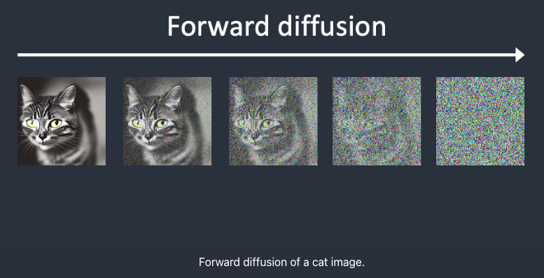
The concept of diffusion begins by adding random noise to an image, let us assume the image to be a cat image. Gradually, by adding noise to the image the image turns to a extremely blurry image which cannot be recognized further. This is called Forward Diffusion.
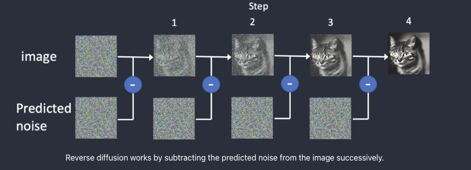
Next, comes the most important part, the Reverse Diffusion. Here, the original image is restored back by removing the noise iteratively. In order to perform Reverse Diffusion, it's essential to understand the amount of noise introduced to an image. This involves training a deep neural network model to predict the added noise, which is referred to as the noise predictor in Stable Diffusion. The noise predictor takes the form of a U-Net model.
The initial step involves creating a random image and using a noise predictor to predict the noise within that image. Subsequently, we subtract this estimated noise from the original image, and this process is iteratively repeated. After a few iterations, the outcome is an image that represents either a cat or a dog.
However, this process is not an efficient process and to speed up the process Latent Diffusion Model is introduced. Stable Diffusion functions as a latent diffusion model. Rather than working within the high-dimensional image space, it initially compresses the image into a latent space. This latent space is 48 times smaller, leading to the advantage of processing significantly fewer numbers. This is the reason for its notably faster performance. Stable Diffusion uses a technique called as the Variational Autoencoder or VAE neural network. This VAE has two parts an encoder and a decoder. The encoder compresses the image into a lower dimensional image and decoder restores the image.
During training, instead of generating noisy images, the model generates tensor in latent space. Instead of introducing noise directly to an image, Stable Diffusion disrupts the image in the latent space with latent noise. This approach is chosen for its efficiency, as operating in the smaller latent space results in a considerably faster process.
However, here we are talking about images now, the question is from where does the text to image comes?
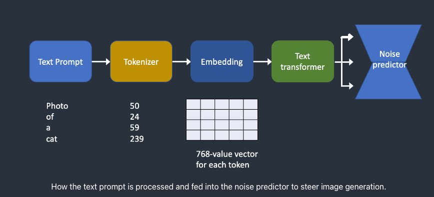
In SDMs, a text prompt is passed to a tokenizer to convert the prompt to tokens or numbers. Tokens are numerical values representing the words and these are used by the computer to understand these words. Each of these tokens are then converted into a 768-value vector called embedding. Next, these embeddings are then processed by the text transformer. At the end the output from the transformers are fed to the Noise Predictor U-Net.
The SD model initiates a random tensor in latent space, this random tensor can be controlled by the seed of the random number generator. This noise is the image in latent space. The Noise predictor takes in this latent noisy image and the prompt and predicts the noise in latent space (4x64x64 tensor).
Furthermore, this latent noise is subtracted from the latent image to generate the new latent image. These steps are iterated which can be adjusted by the sampling steps. Next, the decoder VAE converts the latent image to pixel space, generating the image aligning with the prompt.
Overall, the latent diffusion model combines elements of probability, generative modeling, and diffusion processes to create a framework for generating complex and realistic data from a latent space.
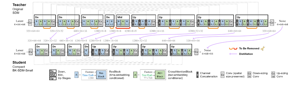
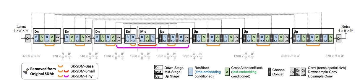
Using Stable Diffusion can be computationally expensive as it involves denoising latents iteratively to generate an image. To reduce the model complexities, the Distilled Stable Diffusion model from Nota AI is introduced. This distilled version streamlines the UNet by removing certain residual and attention blocks of SDM, resulting in a 51% reduction in model size and a 43% improvement in latency on CPU/GPU. This work has been able to achieve greater results and yet being on trained on budget.
As discussed in the research paper , In the Knowledge-distilled SDMs, the U-Net is simplified, which is the most computationally intensive part of the system. The U-Net, embedded by text and time-step information, goes through denoising steps to generate latent representations. The per-step calculations in the U-Net is further minimized, resulting in a more efficient model. The architecture of the model obtained by compressing SDM-v1 is shown in the image below.
Code Demo
Bring this project to life
Click the link provided in this article and navigate to the distilled_stable_diffusion.ipynb notebook. Follow the steps to run the notebook.
Let's begin by installing the required libraries. In addition to the DSD libraries, we will also install Gradio.
!pip install --quiet git+https://github.com/huggingface/diffusers.git@d420d71398d9c5a8d9a5f95ba2bdb6fe3d8ae31f
!pip install --quiet ipython-autotime
!pip install --quiet transformers==4.34.1 accelerate==0.24.0 safetensors==0.4.0
!pip install --quiet ipyplot
!pip install gradio
%load_ext autotime
Next, we will build pipeline and generate the first image and save the generated image.
# Import the necessary libraries

from diffusers import StableDiffusionXLPipeline
import torch
import ipyplot
import gradio as gr

pipe = StableDiffusionXLPipeline.from_pretrained("segmind/SSD-1B", torch_dtype=torch.float16, use_safetensors=True, variant="fp16")
pipe.to("cuda")


prompt = "an orange cat staring off with pretty eyes, Striking image, 8K, Desktop background, Immensely sharp."
neg_prompt = "ugly, poorly Rendered face, low resolution, poorly drawn feet, poorly drawn face, out of frame, extra limbs, disfigured, deformed, body out of frame, blurry, bad composition, blurred, watermark, grainy, signature, cut off, mutation"

image = pipe(prompt=prompt, negative_prompt=neg_prompt).images[0]

image.save("test.jpg")

ipyplot.plot_images([image],img_width=400)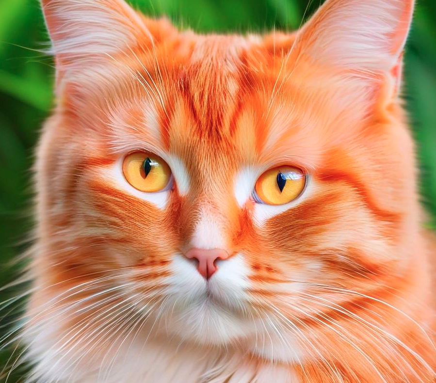
The above code imports the 'StableDiffusionXLPipeline' class from the 'diffusers' module. Post importing the necessary libraries, we will create an instance of the 'StableDiffusionXLPipeline' class named 'pipe.' Next, load the pre-trained model named "segmind/SSD-1B" into the pipeline. The model is configured to use 16-bit floating-point precision that we specify in dtype argument, and safe tensors are enabled. The variant is set to "fp16". Since we will use 'GPU' we will move the pipeline to CUDA device for faster computation.
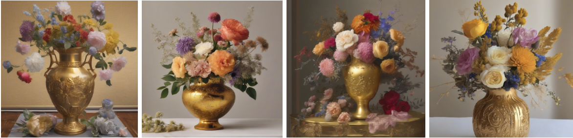
Let us enhance the code further, by adjusting the guidance scale, which impacts the prompts on the image generation. In this case, it is set to 7.5. The parameter 'num_inference_steps' is set to 30, this number indicates the steps to be taken during the image generation process.
allimages = pipe(prompt=prompt, negative_prompt=neg_prompt,guidance_scale=7.5,num_inference_steps=30,num_images_per_prompt=2).images
Build Your Web UI using Gradio
Gradio provides the quickest method to showcase your machine learning model through a user-friendly web interface, enabling accessibility for anyone to use. Let us learn how to built a simple UI using Gradio.
Define a function to generate the images which we will use to built the gradio interface.
def gen_image(text, neg_prompt):
    return pipe(text,
                negative_prompt=neg_prompt,
                guidance_scale=7.5,
                num_inference_steps=30).images[0]
Next, code snippet utilizes the Gradio library to create a simple web interface for generating AI-generated images using a function called gen_image.
txt = gr.Textbox(label="prompt")
txt_2 = gr.Textbox(label="neg_prompt")
Two textboxes (txt and txt_2) are defined using the gr.Textbox class. These textboxes serve as input fields where users can input text data. These fields are used for entering the prompt and the negative prompt.
#Gradio Interface Configuration
demo = gr.Interface(fn=gen_image, inputs=[txt, txt_2], outputs="image", title="Generate A.I. image using Distill Stable Diffusion😁")
demo.launch(share=True)
- First specify the function
gen_imageas the function to be executed when the interface receives input. - Defines the input components for the interface, which are the two textboxes for the prompt and negative prompt (
txtandtxt_2). outputs="image": generate the image output and set the title of the interfacetitle="Generate A.I. image using Distill Stable Diffusion😁"- The
launchmethod is called to start the Gradio interface. Theshare=Trueparameter indicates that the interface should be made shareable, allowing others to access and use it.
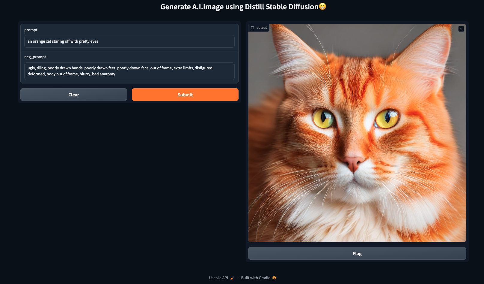
In summary, this code sets up a Gradio interface with two textboxes for user input, connects it to a function (gen_image) for processing, specifies that the output is an image, and launches the interface for sharing. We can input prompts and negative prompts in the textboxes to generate AI-generated images through the provided function.
The SSD-1B model
Recently, Segmind launched the open source foundation model, SSD-1B, and has claimed to be the fastest diffusion text to image model. Developed as a part of the distillation series, SSD-1B shows a 50% reduction in size and a 60% increase in speed when compared with the SDXL 1.0 model. Despite these improvements, there is only a marginal compromise in image quality compared to SDXL 1.0. Additionally, the SSD-1B model has obtained commercial licensing, providing businesses and developers with the opportunity to incorporate this cutting-edge technology into their offerings.
This model is the distilled version of the SDXL, and has proved to generate images of superior quality faster and being affordable at the same time.
The NotaAI/bk-sdm-small
Another distilled version of SD from Nota AI is very common for T2I generations. The Block-removed Knowledge-distilled Stable Diffusion Model (BK-SDM) represents a structurally streamlined version of SDM, designed for efficient general-purpose text-to-image synthesis. Its architecture involves (i) eliminating multiple residual and attention blocks from the U-Net of Stable Diffusion v1.4 and (ii) pretraining through distillation using only 0.22M LAION pairs, which is less than 0.1% of the complete training set. Despite the use of significantly restricted resources in training, this compact model demonstrates the ability to mimic the original SDM through the effective transfer of knowledge.
Is the Distilled Version really fast?
Now, the question arises are these distilled version of SD really fast, and there is only one way to find out. Let us test out 4 models from Stable Diffusions using our Paperspace GPU.
In this evaluation, we will assess four models belonging to the diffusion family. We will be using segmind/SSD-1B, stabilityai/stable-diffusion-xl-base-1.0, nota-ai/bk-sdm-small, CompVis/stable-diffusion-v1-4 for our evaluation purpose. Please feel free to click on the link for a detailed comparative analysis on SSD-1B and SDXL.
Let us load all the models and compare them:
import torch
import time
import ipyplot

from diffusers import StableDiffusionPipeline, StableDiffusionXLPipeline, DiffusionPipeline
In the below code snippet we will use 4 different pre trained model from the Stable Diffusion family and create a pipeline for text to image synthesis.
#text-to-image synthesis pipeline using the "bk-sdm-small" model from nota-ai
distilled = StableDiffusionPipeline.from_pretrained(
"nota-ai/bk-sdm-small", torch_dtype=torch.float16, use_safetensors=True,
).to("cuda")
#text-to-image synthesis pipeline using the "stable-diffusion-v1-4" model from CompVis
original = StableDiffusionPipeline.from_pretrained(
"CompVis/stable-diffusion-v1-4", torch_dtype=torch.float16, use_safetensors=True,
).to("cuda")
#text-to-image synthesis pipeline using the original "stable-diffusion-xl-base-1.0" model from stabilityai
SDXL_Original = DiffusionPipeline.from_pretrained(
"stabilityai/stable-diffusion-xl-base-1.0", torch_dtype=torch.float16,
use_safetensors=True, variant="fp16"
).to("cuda")
#text-to-image synthesis pipeline using the original "SSD-1B" model from segmind
ssd_1b = StableDiffusionXLPipeline.from_pretrained(
"segmind/SSD-1B", torch_dtype=torch.float16, use_safetensors=True,
variant="fp16"
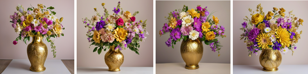
).to("cuda")Once the model is loaded and the pipelines are created we will use these models to generate few images and check the inference time for each of the model.
Please note here that all the model pipelines should not be included in a single cell else one might get into memory issues.
We highly recommend users to click on the link provided to access the entire code.
Bring this project to life
| Model | Inference Time |
|---|---|
| stabilityai/stable-diffusion-xl-base-1.0 | 82212.8 ms |
| segmind/SSD-1B | 59382.0 ms |
| CompVis/stable-diffusion-v1-4 | 15356.6 ms |
| nota-ai/bk-sdm-small | 10027.1 ms |
The bk-sdm-small model took the least amount of inference time, additionally the model was able to generate high quality images.
Concluding thoughts
In this article, we provided a concise overview of the Stable Diffusion model and explored the concept of Distilled Stable Diffusion. Stable Diffusion (SD) emerges as a potent technique for generating new images through straightforward prompts. Additionally, we examined four models within the SD family, highlighting that the bk-sdm-small model demonstrated the shortest inference time. This shows how efficient KD models are compared to the original model.
It is also important to acknowledge that there are certain limitations of the distilled model. Firstly, it doesn't attain flawless photorealism, and legible text rendering is beyond its current capabilities. Moreover, when confronted with complex tasks requiring compositional understanding, the model's performance may drop down. Additionally, facial and general human representations might not be generated accurately. It's crucial to note that the model's training data primarily consists of English captions, which can result in reduced effectiveness when applied to other languages.
Furthermore, to note here that none of the models employed here should be utilized for the generation of disturbing, distressing, or offensive images.
One of the key benefit of distilling these high performing model allows to significantly reduce the computation requirements while generating high quality images.
We encourage our users to try out the links provided in this article to experiment with all of the models using our free GPU. Thanks for reading, we hope you enjoy the model with Paperspace.
References
- Stable Diffusion Paperspace blogs
- Inference with SSD 1B — A distilled Stable Diffusion XL model that is 50% smaller and 60% faster
- Announcing SSD-1B: A Leap in Efficient T2I Generation
- Stable Diffusion pipelines
- Distilled Stable Diffusion inference
- nota-ai/bk-sdm-small
- stabilityai/stable-diffusion-xl-base-1.0
- BK-SDM: A Lightweight, Fast, and Cheap Version of Stable Diffusion