Bring this project to life
One of the issues which plague deep learning models is the fact that they often do not know what they do not know. That being the case models might need an added layer of protection against data classes which they have not been exposed to during training. In this article, we will look at one of such methods in detail.
#  article dependencies
import torch
import torch.nn as nn
import torch.nn.functional as F
import torchvision
import torchvision.transforms as transforms
import torchvision.datasets as Datasets
from torch.utils.data import Dataset, DataLoader
import numpy as np
import matplotlib.pyplot as plt
import cv2
from tqdm.notebook import tqdm
from tqdm import tqdm as tqdm_regular
import seaborn as sns
from torchvision.utils import make_grid
import random
if torch.cuda.is_available():
device = torch.device('cuda:0')
print('Running on the GPU')
else:
device = torch.device('cpu')
print('Running on the CPU')Uncertainty in Deep Learning
Like I had mentioned in the overview, deep learning models often don't know what they don't know. For instance consider a model trained to classify handwritten digits contained in the MNIST dataset, if an image of a table is supplied to said model it will classify this table as either one of the ten handwritten image classes without hesitation. In actual fact, what the model does is to return a vector containing confidence scores for each class and then we have some logic to pick the highest score and classify the image accordingly.
The model has no inherent ability to interject and infer that it has not been exposed to a certain kind of image during training and just goes ahead to treat it as normal. This lack of discernment on the model's part is term uncertainty. When the model acts on out-of-sample data (data from a class not present in the training set) and treats it as normal this is called aleatoric/data uncertainty. However when a model acts on in-sample data but one which is an edge case (looks markedly different from those present in the training set) and treats it as normal this is called epistemic/model uncertainty. There exists ways of measuring these uncertainties, however, this article is focused on how to stop a potential case of aleatoric uncertainty before it happens.
Handing Aleatoric Uncertainty
Handling aleatoric uncertainty in this instance refers to a process of adding some redundancy to our model such that it knows when out-of-sample data is being feed to it. This redundancy will be in the form of another model which has properties making it suitable for detecting out-of-sample data instances. This process can be called anomaly detection, and an obvious candidate for this is a convolutional autoencoder.
Why Convolutional Autoencoders?
As we all know, convolutional autoencoders are deep learning neural networks who's sole purpose is encoding and decoding of input images with the aim of reconstructing them as they were. Just like any other supervised learning task, convolution autoencoders are only suitable for creating reconstructions (even if they are not perfect) of images in classes present in the training set. If an image of a class outside the training set is passed through a convolutional autoencoder, it's reconstruction will be quite unsatisfactory.
Herein lies that property that make convolutional autoencoders suitable for the task of anomaly detection. When a reconstruction is produced, we can measure the reconstruction loss between the original image and the reconstruction then compare this loss with a predefined threshold in a bid to determine if the image is out-of-sample or not.
Implementing an Anomaly Detector
Consider an hypothetical scenario where one intends to train a binary classification model capable of classifying cat and dog images. In this case, in order to serve as an anomaly detector, a convolutional autoencoder needs to be trained to reconstruct only images of cats and dogs. For the sake of this article, those images will be gotten from the CIFAR-10 dataset.
def extract_images(dataset):
  """
  This function extracts images of cats (index 3)
  and dogs (index 5) from the CIFAR-10 dataset.
  """
  cats = []
  dogs = []

  for idx in tqdm_regular(range(len(dataset))):
    if dataset.targets[idx]==3:
      cats.append((dataset.data[idx], 0))
    elif dataset.targets[idx]==5:
      dogs.append((dataset.data[idx], 1))
    else:
      pass
  return cats, dogs


#  loading training data
training_set = Datasets.CIFAR10(root='./', download=True,
                              transform=transforms.ToTensor())

#  loading validation data
validation_set = Datasets.CIFAR10(root='./', download=True, train=False,
                                transform=transforms.ToTensor())


#  extracting training images
cat_train, dog_train = extract_images(training_set)
training_data = cat_train + dog_train
random.shuffle(training_data)

#  extracting validation images
cat_val, dog_val = extract_images(validation_set)
validation_data = cat_val + dog_val
random.shuffle(training_data)


#  removing labels
training_images = [x[0] for x in training_data]
validation_images = [x[0] for x in validation_data]
test_images = [x[0] for x in cat_val[:5]] + [x[0] for x in dog_val[:5]]
Having extracted the images and allotted them to their right objects, it is now time to create a PyTorch dataset which will allow them to be used for training a PyTorch model.
#  defining dataset class
class CustomCIFAR10(Dataset):
  def __init__(self, data, transforms=None):
    self.data = data
    self.transforms = transforms

  def __len__(self):
    return len(self.data)

  def __getitem__(self, idx):
    image = self.data[idx]

    if self.transforms!=None:
      image = self.transforms(image)
    return image


#  creating pytorch datasets
training_data = CustomCIFAR10(training_images, transforms=transforms.Compose([transforms.ToTensor(),
                                                                              transforms.Normalize((0.5, 0.5, 0.5), (0.5, 0.5, 0.5))]))
validation_data = CustomCIFAR10(validation_images, transforms=transforms.Compose([transforms.ToTensor(),
                                                                                  transforms.Normalize((0.5, 0.5, 0.5), (0.5, 0.5, 0.5))]))
test_data = CustomCIFAR10(test_images, transforms=transforms.Compose([transforms.ToTensor(),
                                                                                  transforms.Normalize((0.5, 0.5, 0.5), (0.5, 0.5, 0.5))]))
Convolutional Autoencoder Architecture
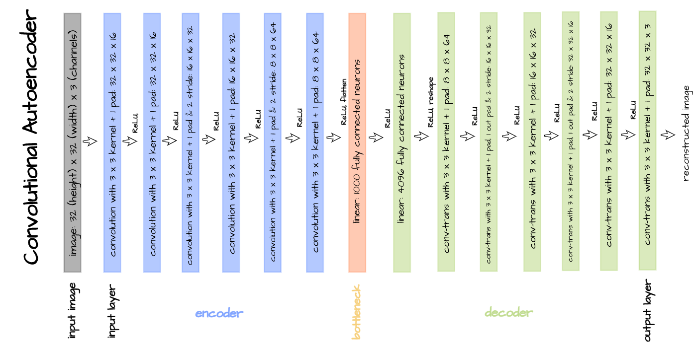
The above illustrated convolutional autoencoder architecture will be implemented for the objectives of this article. Implementation is done by defining the encoder and decoder as distinct classes with the bottleneck attached as the final layer in the encoder. Thereafter, both classes are combined as one in an autoencoder class.
#  defining encoder
class Encoder(nn.Module):
  def __init__(self, in_channels=3, out_channels=16, latent_dim=1000, act_fn=nn.ReLU()):
    super().__init__()

    self.net = nn.Sequential(
        nn.Conv2d(in_channels, out_channels, 3, padding=1), # (32, 32)
        act_fn,
        nn.Conv2d(out_channels, out_channels, 3, padding=1),
        act_fn,
        nn.Conv2d(out_channels, 2*out_channels, 3, padding=1, stride=2), # (16, 16)
        act_fn,
        nn.Conv2d(2*out_channels, 2*out_channels, 3, padding=1),
        act_fn,
        nn.Conv2d(2*out_channels, 4*out_channels, 3, padding=1, stride=2), # (8, 8)
        act_fn,
        nn.Conv2d(4*out_channels, 4*out_channels, 3, padding=1),
        act_fn,
        nn.Flatten(),
        nn.Linear(4*out_channels*8*8, latent_dim),
        act_fn
    )

  def forward(self, x):
    x = x.view(-1, 3, 32, 32)
    output = self.net(x)
    return output


#  defining decoder
class Decoder(nn.Module):
  def __init__(self, in_channels=3, out_channels=16, latent_dim=1000, act_fn=nn.ReLU()):
    super().__init__()

    self.out_channels = out_channels

    self.linear = nn.Sequential(
        nn.Linear(latent_dim, 4*out_channels*8*8),
        act_fn
    )

    self.conv = nn.Sequential(
        nn.ConvTranspose2d(4*out_channels, 4*out_channels, 3, padding=1), # (8, 8)
        act_fn,
        nn.ConvTranspose2d(4*out_channels, 2*out_channels, 3, padding=1,
                           stride=2, output_padding=1), # (16, 16)
        act_fn,
        nn.ConvTranspose2d(2*out_channels, 2*out_channels, 3, padding=1),
        act_fn,
        nn.ConvTranspose2d(2*out_channels, out_channels, 3, padding=1,
                           stride=2, output_padding=1), # (32, 32)
        act_fn,
        nn.ConvTranspose2d(out_channels, out_channels, 3, padding=1),
        act_fn,
        nn.ConvTranspose2d(out_channels, in_channels, 3, padding=1)
    )

  def forward(self, x):
    output = self.linear(x)
    output = output.view(-1, 4*self.out_channels, 8, 8)
    output = self.conv(output)
    return output


#  defining autoencoder
class Autoencoder(nn.Module):
  def __init__(self, encoder, decoder):
    super().__init__()
    self.encoder = encoder
    self.encoder.to(device)

    self.decoder = decoder
    self.decoder.to(device)

  def forward(self, x):
    encoded = self.encoder(x)
    decoded = self.decoder(encoded)
    return decoded
Convolutional Neural Network Class
The class below is defined to combine training, validation as well as other functionalities of our convolutional autoencoder.
class ConvolutionalAutoencoder():
  def __init__(self, autoencoder):
    self.network = autoencoder
    self.optimizer = torch.optim.Adam(self.network.parameters(), lr=1e-3)

  def train(self, loss_function, epochs, batch_size,
            training_set, validation_set, test_set):

    #  creating log
    log_dict = {
        'training_loss_per_batch': [],
        'validation_loss_per_batch': [],
        'visualizations': []
    }

    #  defining weight initialization function
    def init_weights(module):
      if isinstance(module, nn.Conv2d):
        torch.nn.init.xavier_uniform_(module.weight)
        module.bias.data.fill_(0.01)
      elif isinstance(module, nn.Linear):
        torch.nn.init.xavier_uniform_(module.weight)
        module.bias.data.fill_(0.01)

    #  initializing network weights
    self.network.apply(init_weights)

    #  creating dataloaders
    train_loader = DataLoader(training_set, batch_size)
    val_loader = DataLoader(validation_set, batch_size)
    test_loader = DataLoader(test_set, 10)

    #  setting convnet to training mode
    self.network.train()
    self.network.to(device)

    for epoch in range(epochs):
      print(f'Epoch {epoch+1}/{epochs}')
      train_losses = []

      #------------
      #  TRAINING
      #------------
      print('training...')
      for images in tqdm(train_loader):
        #  zeroing gradients
        self.optimizer.zero_grad()
        #  sending images to device
        images = images.to(device)
        #  reconstructing images
        output = self.network(images)
        #  computing loss
        loss = loss_function(output, images.view(-1, 3, 32, 32))
        #  calculating gradients
        loss.backward()
        #  optimizing weights
        self.optimizer.step()

        #--------------
        # LOGGING
        #--------------
        log_dict['training_loss_per_batch'].append(loss.item())

      #--------------
      # VALIDATION
      #--------------
      print('validating...')
      for val_images in tqdm(val_loader):
        with torch.no_grad():
          #  sending validation images to device
          val_images = val_images.to(device)
          #  reconstructing images
          output = self.network(val_images)
          #  computing validation loss
          val_loss = loss_function(output, val_images.view(-1, 3, 32, 32))

        #--------------
        # LOGGING
        #--------------
        log_dict['validation_loss_per_batch'].append(val_loss.item())


      #--------------
      # VISUALISATION
      #--------------
      print(f'training_loss: {round(loss.item(), 4)} validation_loss: {round(val_loss.item(), 4)}')

      for test_images in test_loader:
        #  sending test images to device
        test_images = test_images.to(device)
        with torch.no_grad():
          #  reconstructing test images
          reconstructed_imgs = self.network(test_images)
        #  sending reconstructed and images to cpu to allow for visualization
        reconstructed_imgs = reconstructed_imgs.cpu()
        test_images = test_images.cpu()

        #  visualisation
        imgs = torch.stack([test_images.view(-1, 3, 32, 32), reconstructed_imgs],
                          dim=1).flatten(0,1)
        grid = make_grid(imgs, nrow=10, normalize=True, padding=1)
        grid = grid.permute(1, 2, 0)
        plt.figure(dpi=170)
        plt.title('Original/Reconstructed')
        plt.imshow(grid)
        log_dict['visualizations'].append(grid)
        plt.axis('off')
        plt.show()

    return log_dict

  def autoencode(self, x):
    return self.network(x)

  def encode(self, x):
    encoder = self.network.encoder
    return encoder(x)

  def decode(self, x):
    decoder = self.network.decoder
    return decoder(x)
Training and Validation
Bring this project to life
With everything in the right order, it is now time to train our convolutional autoencoder. The autoencoder is trained with parameters as defined in the code cell below.
# training model
model = ConvolutionalAutoencoder(Autoencoder(Encoder(), Decoder()))
log_dict = model.train(nn.MSELoss(), epochs=30, batch_size=64,
training_set=training_data, validation_set=validation_data,
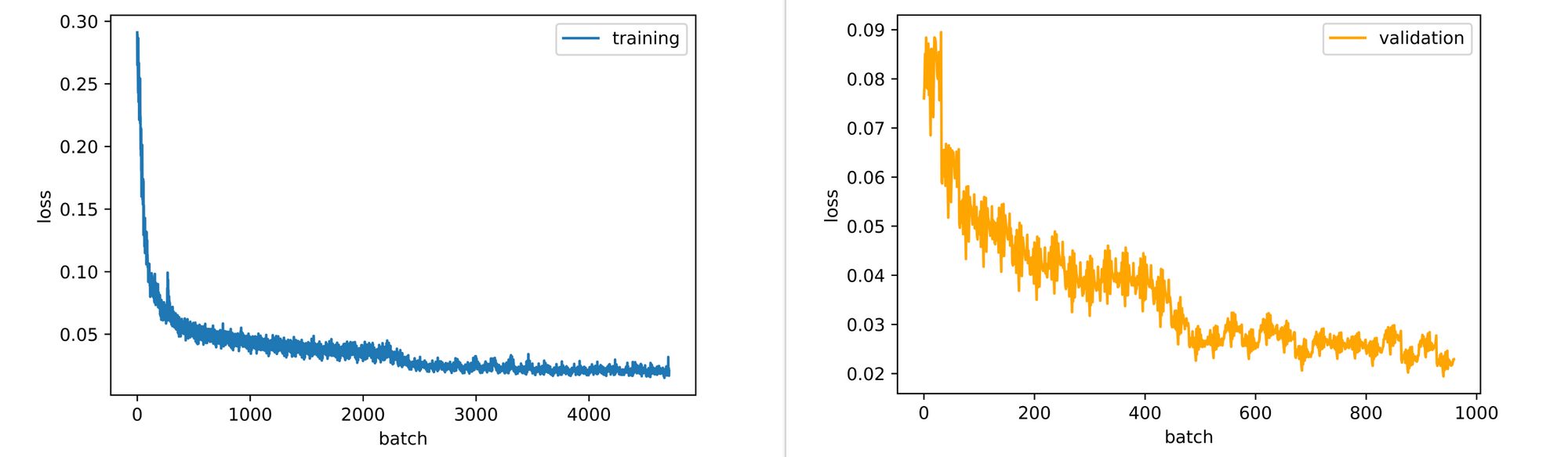
test_set=test_data)From the visualizations and losses returned at the end of each epoch, it can be seen that the autoencoder gradually learns how to reconstruct images even if they are still blurry at the end of the 30th epoch (feel free to train for longer).
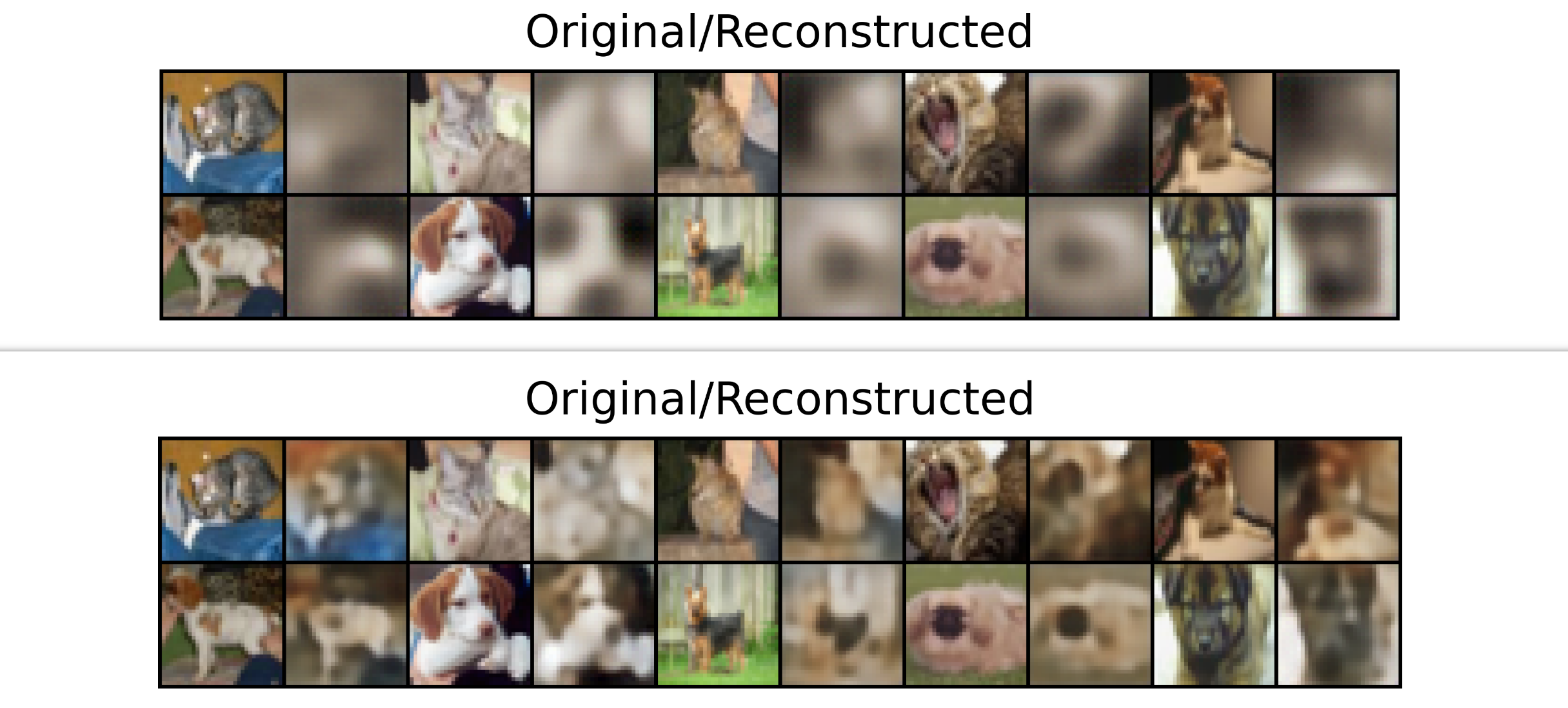
Also, the training and validation loss plots are still slightly down-trending so the model might benefit from some extra epochs of training.
Computing Reconstruction Loss
The function below accepts an image as parameter then proceeds to pass said image through the already trained convolutional autoencoder in order to derive a reconstruction of the image. Thereafter, mean squared error is used to measure reconstruction loss between the uploaded image and it's reconstruction. Using this function we will be deriving reconstruction loss for some images in a bid to determine a possible baseline for out-of-sample data (anomalies).
def reconstruction_loss(image, model, visualize=True):
  """
  This function calculates the reconstruction loss of an
  image for anomaly detection
  """
  #  reading image
  image = cv2.imread(image)
  image = cv2.cvtColor(image, cv2.COLOR_BGR2RGB)
  image = cv2.resize(image, (32, 32))

  #  defining transforms
  transform =transforms.Compose([transforms.ToTensor(),
                                 transforms.Normalize((0.5, 0.5, 0.5), (0.5, 0.5, 0.5))])
  image = transform(image)
  image = image.view(-1, 3, 32, 32)
  image = image.to(device)

  #  passing image through autoencoder
  with torch.no_grad():
    reconstruction = model.autoencode(image)
    #  computing reconstruction loss
    reconstruction_loss = F.mse_loss(image, reconstruction)

  print(f'reconstruction_loss: {round(reconstruction_loss.item(), 4)}')

  if visualize:
    #  visualization
    grid = make_grid([image.view(3, 32, 32).cpu(), reconstruction.view(3, 32, 32).cpu()], normalize=True, padding=1)
    grid = grid.permute(1,2,0)
    plt.figure(dpi=100)
    plt.title('uploaded/reconstruction')
    plt.axis('off')
    plt.imshow(grid)
  else:
    pass

  return round(reconstruction_loss.item(), 4)
Cat Image 1
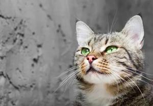
With regards to the cat image above, when passed through the autoencoder we expect it to be reasonably reconstructed so we expect a low reconstruction loss. A reconstruction loss of 0.04 is returned but we need more samples before we can define a baseline close to that value.
#  computing loss
recon_loss = reconstruction_loss('cat_1.jpg', model=model)

# >>> reconstruction_loss: 0.0447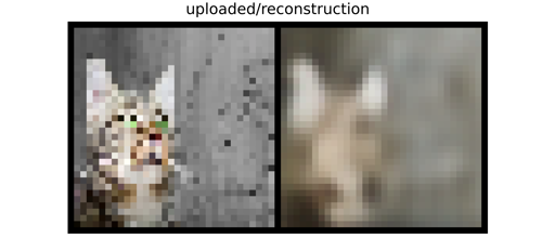
Cat Image 2

Just to be sure, let's try another cat image to see how well the autoencoder reconstructs the image. Upon passing a new cat image through the autoencoder, a reconstruction loss of approximately 0.02 is returned, lower than the first image.
#  computing loss
recon_loss = reconstruction_loss('cat_2.jpg', model=model)

# >>> reconstruction_loss: 0.0191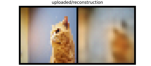
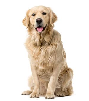
Dog Image 1
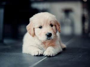
Since the convolutional autoencoder is trained to reconstruct both cat and dog images then we are required to check it's reconstruction of dog images as well. When the image above is passed through the autoencoder a reconstruction loss of about 0.04 is again returned, similar to the first cat image.
#  computing loss
recon_loss = reconstruction_loss('dog_1.jpg', model=model)

# >>> reconstruction_loss: 0.0354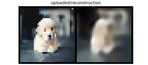
Dog Image 2
Keeping with the theme, again let's try our model on another dog image, the one illustrated above. Upon passing this image through the autoencoder, a reconstruction loss of approximately 0.04 is returned, a same as two of the last 3 images.
#  computing loss
recon_loss = reconstruction_loss('dog_2.jpg', model=model)

# >>> reconstruction_loss: 0.0399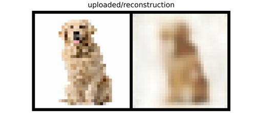
Out-of-Sample image 1
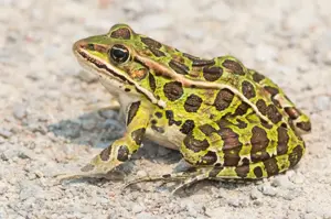
Already, we are getting a sense that the autoencoder reconstructs in-sample images with a loss of 0.04 so a reconstruction loss of around 0.045 - 0.05 will be a decent baseline. However, before we jump into conclusions, we might as well check the autoencoder against out-of-sample images. Using the frog image above we can see that the function outputs a reconstruction loss of 0.07 which is considerably higher than any of the in-sample images.
#  computing loss
recon_loss = reconstruction_loss('out_of_sample_1.jpg', model=model)

# >>> reconstruction_loss: 0.0726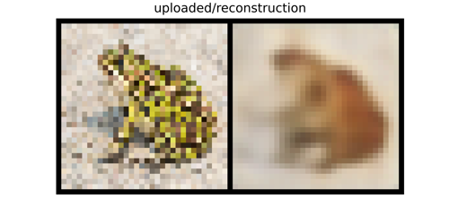
Out-of-Sample Image 2

Testing the autoencoder against another out of sample image yields a reconstruction loss of 0.06. Again, considerably higher than for in-sample images.
#  computing loss
recon_loss = reconstruction_loss('out_of_sample_2.jpg', model=model)

# >>> reconstruction_loss: 0.0581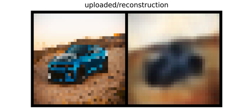
Out-of-Sample Image 3
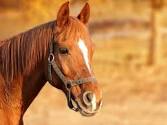
However it should be noted that anomaly detection with convolutional autoencoders is not always a full proof technique. Typical to other models in deep learning, autoencoders are also susceptible to error. Consider the case of the horse image above, a reconstruction loss of about 0.04 is returned, similar to in-sample images even though this is clearly an out-of-sample image.
#  computing loss
recon_loss = reconstruction_loss('out_of_sample_3.jpg', model=model)

# >>> reconstruction_loss: 0.037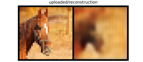
Utilizing the Anomaly Detector
Now that the anomaly detector has been trained and a suitable baseline established (we are selecting 0.045 in this case), we can then proceed to use it as a screen for aleatoric uncertainty. To do this, a function needs to be written such that any image which is supplied to the model for classification purposes first passes through the anomaly detector and satisfies the baseline reconstruction loss before being supplied unto the model for classification purposes.
def aleatoric_screen(image, model):
  """
  This function calculates the reconstruction loss of an
  image and acts as a screen against out-of-sample images
  """
  #  reading image
  image = cv2.imread(image)
  image = cv2.cvtColor(image, cv2.COLOR_BGR2RGB)
  image = cv2.resize(image, (32, 32))

  #  defining transforms
  transform =transforms.Compose([transforms.ToTensor(),
                                 transforms.Normalize((0.5, 0.5, 0.5), (0.5, 0.5, 0.5))])
  image = transform(image)
  image = image.view(-1, 3, 32, 32)
  image = image.to(device)

  #  passing image through autoencoder
  with torch.no_grad():
    reconstruction = model.autoencode(image)
    #  computing reconstruction loss
    reconstruction_loss = F.mse_loss(image, reconstruction)
    reconstruction_loss = round(reconstruction_loss.item(), 3)

  if reconstruction_loss > 0.045:
    print('The model is not built to classify this sort of image')
  else:
    return image
Final Remarks
In this article, we took a brief look at uncertainties in deep learning. Thereafter, we took a more keen look at aleatoric uncertainty and how convolutional autoencoder can help to screen out-of-sample images for classification tasks.