Bring this project to life
Introduction
This paper was a significant step forward in applying the attention mechanism, serving as the primary development for a model known as the transformer. The most well-known models currently being developed for NLP tasks consist of many transformers. In this tutorial, we will outline the components of this model.
The reason why we need transformers
First-generation approaches for neural machine translation, which use RNNs in an encoder-decoder architecture, were centered on using RNNs for sequence-to-sequence challenges.
When dealing with extended sequences, these designs had a significant shortcoming; their capacity to preserve information from the initial components was lost when additional elements were introduced into the sequence. There is a hidden state for each step in the encoder, which is generally tied to one of the most recent input words. Consequently, if the decoder only accesses the latest hidden state of the encoder, it will lose information about the earlier components of the sequence. As a solution to this problem, a new concept was introduced: Attention Mechanisms.
While RNNs often focus on an encoder's last state, we look at all the encoder's states during decoding, allowing us to obtain information about every element in an input sequence. This is what attention does: it compiles a weighted sum of all previous encoder states from the whole sequence.
As a result, the decoder might prioritize particular input elements for each element of the output. Learning to anticipate the next output element by focusing on the correct input element at each stage.
It is, nevertheless, crucial to note that this strategy still has a significant limitation: each sequence must be processed individually. To process the t-th step, both the encoder and the decoder must wait for the previous t-1 steps to complete. Because of this, it takes a long time and uses a lot of computing power to process large datasets.
A few Types of Attention
Hard and soft Attention
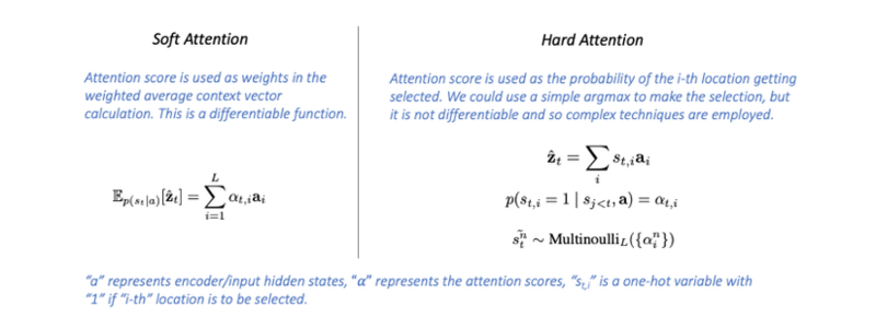
As mentioned by Luong et al. in their article and detailed by Xu et al. in their paper, Soft attention occurs when we compute the context vector as a weighted sum of the encoder hidden states. Hard Attention occurs when, in place of a weighted average of all hidden states, we pick a single hidden state based on the attention scores. The selection is an issue since we could make it using a function like argmax, but because that function is not differentiable, more advanced training strategies are required.
Global Attention
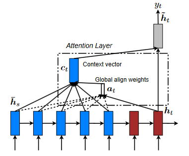
The term "global attention" refers to the situation in which ALL encoder hidden states are used to build the attention-based context vector for each decoder step.
As you may have imagined, this might quickly become costly. A global attentional model considers all the encoder's hidden states when deriving the context vector (ct). A variable-length alignment vector at, the size of which is equal to the number of time steps on the source side, is derived in this model type by comparing the current target hidden state ht with each source hidden state hs.
Local Attention
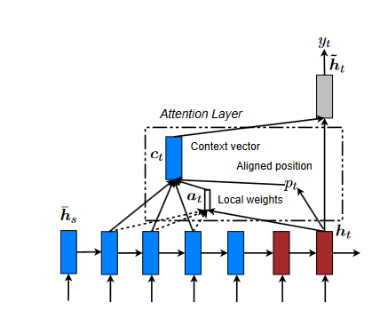
The disadvantage of using global attention is that it must pay attention to all words on the source side for each term on the target side. It is not only time-consuming and labor-intensive, but it also has the potential to make it impractical to translate longer sequences, such as paragraphs or documents. We suggest using a local attentional mechanism as a solution to this problem. This mechanism would concentrate only on a tiny subset of the source locations associated with each target word.
Xu et al.(2015) proposal's tradeoff between soft and hard attentional models served as a source of motivation for developing this model to solve the challenge of generating image captions. Within their research, "soft attention" refers to the global attention technique, characterized by the "gentle" application of weights over all of the source image's patches.
On the other hand, the hard attention method focuses on a single portion of the image at a time. To train a hard attention model, one must use more complex techniques like variance reduction or reinforcement learning, even though they are less expensive at inference time. Our local attention mechanism focuses selectively on a narrow context window and is differentiable. This strategy has the benefit of avoiding the costly computation incurred in the soft attention approach, and at the same time, it is simpler to train than the hard attention approach. The model starts by generating an aligned position denoted by pt, for each target word at the given time t.
After that, the context vector, denoted by ct, is generated by taking a weighted average over the source hidden states inside the window [pt−D, pt+D]; D is empirically selected. In contrast to the global method, the local alignment vector at is now of a fixed dimension. There are two possibilities for the model, which are outlined below:
- Monotonic alignment (local-m): We set pt = t on the assumption that the source and target sequences are approximately monotonically aligned.
- Predictive alignment (local-p): Rather than assuming a monotonic aligned position, our model predicts an aligned position:
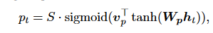
The model parameters wp and vp will be learned to make position predictions.
The length of the source sentence is denoted by "S." pt falls in the range [0, S] as a direct consequence of the sigmoid function. We establish a Gaussian distribution centered around pt to prefer alignment points close to pt.
Latent Attention
Translating natural language descriptions into executable programs is a key topic in computational linguistics. The natural language processing and programming language communities have been working on this topic for the last decade. For the sake of this study, researchers are only interested in subsets programs with one if-then expression. Recipes are If-Then programs that provide a trigger condition and an action function, and they represent programs that execute when the trigger is fulfilled.
An LSTM technique, a neural network, and logistic regression approaches have been presented to solve this problem. On the other hand, the authors contend that the wide variety of vocabulary and sentence patterns makes it impossible for an RNN to learn usable representations, and their ensemble technique does outperform the LSTM-based approach on the function predictions challenge. As a solution, the authors provide a novel attention architecture they term Latent Attention. Latent attention uses a weighting system to assess the importance of each token in predicting the trigger or the action.
Latent Attention Model
If we want to turn a natural language description into a program, we need to find the terms in the description that are most useful in predicting the intended labels. An illustration of this is provided in the following description:
Autosave Instagram photos to your Dropbox folder
The term "Instagram photos" is the one that is going to help us predict the trigger the best. To get this information, we can adapt the attention mechanism such that it first computes a weight based on the importance of each token in the sentence and then outputs a weighted sum of the embeddings of these tokens. On the other hand, our gut feeling tells us that each token's importance is determined by the token itself and the structure of the whole sentence. As an example, if we consider the following sentence:
Post photos in your Dropbox folder to Instagram.
"Dropbox" is used to decide the trigger, although "Instagram" should have played this role in the preceding example, which includes practically identical set of tokens. In this example, the use of prepositions such as "to" gives the impression that the trigger channel is described somewhere in the midst of the process rather than the end. Considering all this enables us to choose "Dropbox" over "Instagram."
We use the standard attention mechanism to compute a latent weight for each token to identify which tokens in the sequence are more relevant to the trigger or action. The final attention weights, which we will refer to as the active weights, are determined by the latent weights. For example, if the token "to" is already present in the expression, we may search for the trigger by looking at the tokens that came before "to.
What is the Transformer?
According to the paper, the transformer is a model architecture that forgoes the use of recurrence in favor of depending only on an attention mechanism to determine global interdependence between input and output. After being trained for as little as twelve hours on eight P100 GPUs, the transformer is capable of reaching a new state of the art in translation quality and allowing for a significant increase in parallelization. The transformer is the first transduction model that computes representations of its input and output only via self-attention rather than sequence-aligned RNNs or convolution.
Word embedding
An embedding is a representation of a symbol (word, character, or phrase) in a distributed low-dimensional space of continuous-valued vectors. Words are not individual symbols. They have a significant and positive relationship with one another. Because of this, we can discover affinities between them when we project them into a continuous Euclidean space. Then, depending on the job, we may space out the word embeddings or keep them relatively near one another.
Model Architecture
Most competitive neural sequence transduction models have an encoder-decoder structure. Here, the encoder maps an input sequence of symbol representations (x1, ..., xn) to a sequence of continuous representations z = (z1, ..., zn). Given z, the decoder then generates an output sequence (y1, ..., ym) of symbols one element at a time. At each step, the model is auto-regressive, consuming the previously generated symbols as additional input when generating the next.
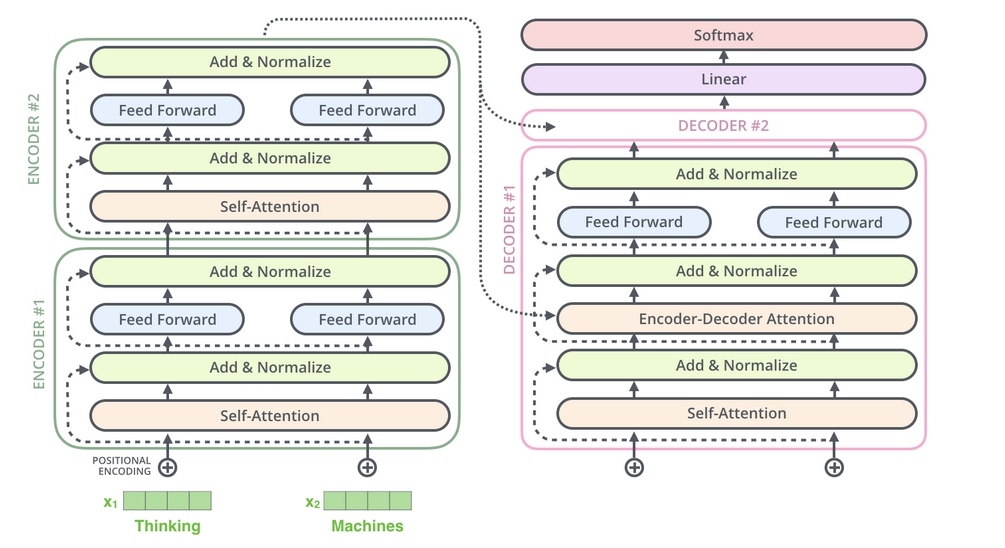
We can see here that the encoder model is on the left, while the decoder is on the right. Attention and feed-forward networks can be found in both blocks.
Self-Attention: the fundamental operation
According to this article, self-attention is a sequence-to-sequence operation. It means that a series of vectors are fed into the process, and another sequence of vectors comes out. Let's refer to the input vectors as x1, x2,..., and xt, and the output vectors as y1, y2,..., and yt. The self-attention operation consists of nothing more than taking a weighted average across all of the input vectors to obtain the output vector yi.
j indexes over the whole sequence and the weights sum to one over all j. The weight wij is not a parameter, as in a normal neural net, but it is derived from a function over 𝐱i and 𝐱j. The simplest option for this function is the dot product.
We must include the following three components in the self-attention mechanism of our model: Queries, Values, and Keys.
The Query, The Value, and The Key
Information retrieval systems are the source of key-value-query concepts. Clarifying these concepts will be tremendously beneficial, and it would be highly beneficial to spell out these key terms. Using YouTube as an example, let's look at how to find a video.
Your search (query) for a particular video will cause the search engine to map your search against a set of keys (video title, description, and so on) that are related to probable videos that have been stored. Then, the algorithm will show you the videos closest to what you're looking for (values). To draw the transformer's attention to this concept, we have the following:
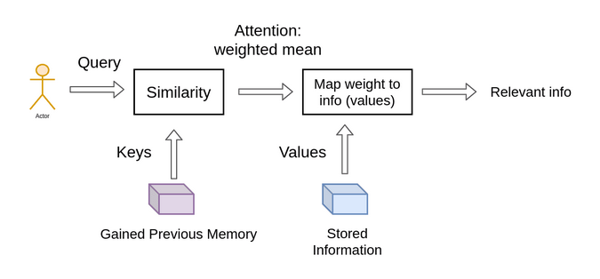
While retrieving a single video, we focused on selecting the video with the highest possible relevance score. The most critical distinction between attention and retrieval systems is that we provide a concept of "retrieving" an item that is more abstract and streamlined. We can weight our query by first determining the degree of similarity, or weight, that exists between our representations. So, taking another step further, we split the data into key-value pairs and use the keys to determine the attention weights to look at the values and the data as the information we will acquire.
Bring this project to life
The Scaled Dot-Product Attention
The name we've given to this specific attention is "Scaled Dot-Product Attention." The input includes:
- queries,
- keys of dimension dk,
- values of dimension dv.
To obtain the weights on the values, we first compute the dot products of the query with all keys, divide each by √dk, and then apply a softmax function. In actual practice, we compute the attention function on a collection of queries all at once and then pack those queries into a matrix Q. The keys and values are also bundled together into matrices K and V. The scores indicate how much weight should be given to other locations or words in the input sequence relative to a particular word at a specific position. To clarify, it would be the dot product of the query vector and the key vector of the corresponding word that is being scored. Therefore, to get the dot product (.) for position 1, we first compute q1.k1, followed by q1.k2, q1.k3, and so on...
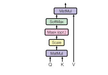
For more stable gradients, we apply the "scaled" factor. It is worth noting that the softmax function cannot perform correctly with large values, leading to the gradients' vanishing and a slowdown in the learning process. After that, we use the Value matrix to maintain the values of the words we want to concentrate on and reduce or remove the values for the words that are unnecessary to our purpose.

def scaled_dot_product_attention(queries, keys, values, mask):
    # Calculate the dot product, QK_transpose
    product = tf.matmul(queries, keys, transpose_b=True)
    # Get the scale factor
    keys_dim = tf.cast(tf.shape(keys)[-1], tf.float32)
    # Apply the scale factor to the dot product
    scaled_product = product / tf.math.sqrt(keys_dim)
    # Apply masking when it is requiered
    if mask is not None:
        scaled_product += (mask * -1e9)
    # dot product with Values
    attention = tf.matmul(tf.nn.softmax(scaled_product, axis=-1), values)

    return attention
Multi-head Attention
Even if two sentences have the same words but are organized in a different order, the attention scores would still provide the same results. Consequently, we'd want to focus on different parts of the words.
The simplest way to understand multi-head self-attention is to see it as a small number of copies of the self-attention mechanism applied in parallel, each with their own key, value, and query transformation.
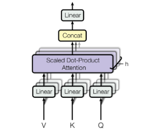
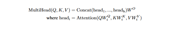
The model can attend to information from different representation subspaces at different points using multi-head attention. It is possible to enhance the ability of the self-attention to differentiate between different words by breaking the word vectors into a defined number of chunks and then applying the self-attention to the corresponding chunks, using Q, K, and V sub-matrices. Once we've calculated the dot product of each head, we concatenate the output matrices and multiply them by a weights matrix.
class MultiHeadAttention(layers.Layer):

    def __init__(self, n_heads):
        super(MultiHeadAttention, self).__init__()
        self.n_heads = n_heads

    def build(self, input_shape):
        self.d_model = input_shape[-1]
        assert self.d_model % self.n_heads == 0
        # Calculate the dimension of every head or projection
        self.d_head = self.d_model // self.n_heads
        # Set the weight matrices for Q, K and V
        self.query_lin = layers.Dense(units=self.d_model)
        self.key_lin = layers.Dense(units=self.d_model)
        self.value_lin = layers.Dense(units=self.d_model)
        # Set the weight matrix for the output of the multi-head attention W0
        self.final_lin = layers.Dense(units=self.d_model)

    def split_proj(self, inputs, batch_size): # inputs: (batch_size, seq_length, d_model)
        # Set the dimension of the projections
        shape = (batch_size,
                 -1,
                 self.n_heads,
                 self.d_head)
        # Split the input vectors
        splited_inputs = tf.reshape(inputs, shape=shape) # (batch_size, seq_length, nb_proj, d_proj)
        return tf.transpose(splited_inputs, perm=[0, 2, 1, 3]) # (batch_size, nb_proj, seq_length, d_proj)

    def call(self, queries, keys, values, mask):
        # Get the batch size
        batch_size = tf.shape(queries)[0]
        # Set the Query, Key and Value matrices
        queries = self.query_lin(queries)
        keys = self.key_lin(keys)
        values = self.value_lin(values)
        # Split Q, K y V between the heads or projections
        queries = self.split_proj(queries, batch_size)
        keys = self.split_proj(keys, batch_size)
        values = self.split_proj(values, batch_size)
        # Apply the scaled dot product
        attention = scaled_dot_product_attention(queries, keys, values, mask)
        # Get the attention scores
        attention = tf.transpose(attention, perm=[0, 2, 1, 3])
        # Concat the h heads or projections
        concat_attention = tf.reshape(attention,
                                      shape=(batch_size, -1, self.d_model))
        # Apply W0 to get the output of the multi-head attention
        outputs = self.final_lin(concat_attention)

        return outputs
Positional Encoding
Having no recurrence and no convolution in our model, it is necessary to provide some information on how tokens are positioned in relation to each other inside the sequence. "Positional Encodings" are added to the embeddings at the bottom of the encoder and decoder stacks to achieve this goal. Because the positional encodings and the embeddings each have the same dimension, it is possible to add up both values. We then use a function to transform the position in the sentence into a real-valued vector. Eventually, the network will figure out how to use this information.
A position embedding might be used like word embedding, where every known position is coded with a vector. In the paper, sine and cosine functions is applied:
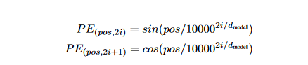
The authors of the transformer study came up with a sinusoidal function for positional encoding in the transformer paper itself. The sine function instructs the model to focus on a specific wavelength. The wavelength of a signal y(x)=sin(kx) is k=2π/λ. λ will be determined by the sentence's position. The value i indicates whether a position is odd or even.
class PositionalEncoding(layers.Layer):

    def __init__(self):
        super(PositionalEncoding, self).__init__()

    def get_angles(self, pos, i, d_model): # pos: (seq_length, 1) i: (1, d_model)
        angles = 1 / np.power(10000., (2*(i//2)) / np.float32(d_model))
        return pos * angles # (seq_length, d_model)

    def call(self, inputs):
        # input shape batch_size, seq_length, d_model
        seq_length = inputs.shape.as_list()[-2]
        d_model = inputs.shape.as_list()[-1]
        # Calculate the angles given the input
        angles = self.get_angles(np.arange(seq_length)[:, np.newaxis],
                                 np.arange(d_model)[np.newaxis, :],
                                 d_model)
        # Calculate the positional encodings
        angles[:, 0::2] = np.sin(angles[:, 0::2])
        angles[:, 1::2] = np.cos(angles[:, 1::2])
        # Expand the encodings with a new dimension
        pos_encoding = angles[np.newaxis, ...]

        return inputs + tf.cast(pos_encoding, tf.float32)
The Encoder
The paper introduces the encoder components as follows:
- The encoder comprises a stack with N = 6 layers that are identical.
- Each layer has two sub-layers. The first is a multi-head self-attention mechanism, and the second is a fully connected feed-forward network.
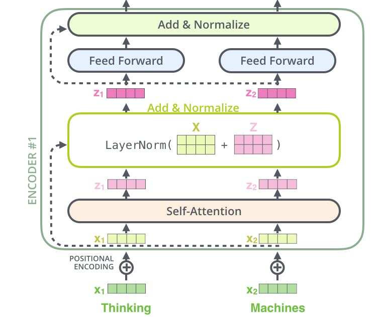
- The residual connection is used around each of the two sub-layers, followed by layer normalization. The output of each sub-layer is LayerNorm(x + Sublayer(x)), where Sublayer(x) is the function implemented by the sub-layer itself.
Normalization and residual connections are two of the most common techniques used to speed up and improve the accuracy of deep neural network training. Only the embedding dimension is affected by the layer normalization. For each sub-layer, we apply dropout on the output before normalizing and combining it with the sub-layer input. Both the encoder and decoder stack embedding and positional encoding sums are dropped out.
We're not using Batch Normalization since it requires much GPU RAM. BatchNorm has been proven to perform especially poorly in language because the features of words tend to have a significantly higher variance (many scarce words need to be considered for a reasonable distribution estimate).
Note: As with ResNets, Transformers also tend to go deep. More than 24 blocks may be found in specific models. A smooth gradient flow can only occur if the model has residual connections. We will proceed with the implementation of encoder layer:
class EncoderLayer(layers.Layer):

    def __init__(self, FFN_units, n_heads, dropout_rate):
        super(EncoderLayer, self).__init__()
        # Hidden units of the feed forward component
        self.FFN_units = FFN_units
        # Set the number of projectios or heads
        self.n_heads = n_heads
        # Dropout rate
        self.dropout_rate = dropout_rate

    def build(self, input_shape):
        self.d_model = input_shape[-1]
        # Build the multihead layer
        self.multi_head_attention = MultiHeadAttention(self.n_heads)
        self.dropout_1 = layers.Dropout(rate=self.dropout_rate)
        # Layer Normalization
        self.norm_1 = layers.LayerNormalization(epsilon=1e-6)
        # Fully connected feed forward layer
        self.ffn1_relu = layers.Dense(units=self.FFN_units, activation="relu")
        self.ffn2 = layers.Dense(units=self.d_model)
        self.dropout_2 = layers.Dropout(rate=self.dropout_rate)
        # Layer normalization
        self.norm_2 = layers.LayerNormalization(epsilon=1e-6)

    def call(self, inputs, mask, training):
        # Forward pass of the multi-head attention
        attention = self.multi_head_attention(inputs,
                                              inputs,
                                              inputs,
                                              mask)
        attention = self.dropout_1(attention, training=training)
        # Call to the residual connection and layer normalization
        attention = self.norm_1(attention + inputs)
        # Call to the FC layer
        outputs = self.ffn1_relu(attention)
        outputs = self.ffn2(outputs)
        outputs = self.dropout_2(outputs, training=training)
        # Call to residual connection and the layer normalization
        outputs = self.norm_2(outputs + attention)

        return outputs
And the encoder implementation:
class Encoder(layers.Layer):

    def __init__(self,
                 n_layers,
                 FFN_units,
                 n_heads,
                 dropout_rate,
                 vocab_size,
                 d_model,
                 name="encoder"):
        super(Encoder, self).__init__(name=name)
        self.n_layers = n_layers
        self.d_model = d_model
        # The embedding layer
        self.embedding = layers.Embedding(vocab_size, d_model)
        # Positional encoding layer
        self.pos_encoding = PositionalEncoding()
        self.dropout = layers.Dropout(rate=dropout_rate)
        # Stack of n layers of multi-head attention and FC
        self.enc_layers = [EncoderLayer(FFN_units,
                                        n_heads,
                                        dropout_rate)
                           for _ in range(n_layers)]

    def call(self, inputs, mask, training):
        # Get the embedding vectors
        outputs = self.embedding(inputs)
        # Scale the embeddings by sqrt of d_model
        outputs *= tf.math.sqrt(tf.cast(self.d_model, tf.float32))
        # Positional encodding
        outputs = self.pos_encoding(outputs)
        outputs = self.dropout(outputs, training)
        # Call the stacked layers
        for i in range(self.n_layers):
            outputs = self.enc_layers[i](outputs, mask, training)

        return outputs
Decoder
The encoder and the decoder both include some of the same components, but those components are employed differently in the decoder so that it can consider the encoder's output.
- The decoder is also composed of a stack of N = 6 identical layers.
- In addition to the two sub-layers in each encoder layer, the decoder inserts a third sub-layer, which performs multi-head attention over the output of the encoder stack.
- Like the encoder, residual connections are used around each sub-layers, followed by layer normalization.
- The self-attention sub-layer is modified in the decoder stack to prevent positions from attending to subsequent positions. This masking, in conjunction with the fact that the output embeddings are shifted by one position, guarantees that the predictions for position i can only rely on the outputs known to occur at positions lower than i.
Decoder Layer implementation:
class DecoderLayer(layers.Layer):

    def __init__(self, FFN_units, n_heads, dropout_rate):
        super(DecoderLayer, self).__init__()
        self.FFN_units = FFN_units
        self.n_heads = n_heads
        self.dropout_rate = dropout_rate

    def build(self, input_shape):
        self.d_model = input_shape[-1]

        # Self multi head attention, causal attention
        self.multi_head_causal_attention = MultiHeadAttention(self.n_heads)
        self.dropout_1 = layers.Dropout(rate=self.dropout_rate)
        self.norm_1 = layers.LayerNormalization(epsilon=1e-6)

        # Multi head attention, encoder-decoder attention
        self.multi_head_enc_dec_attention = MultiHeadAttention(self.n_heads)
        self.dropout_2 = layers.Dropout(rate=self.dropout_rate)
        self.norm_2 = layers.LayerNormalization(epsilon=1e-6)

        # Feed foward
        self.ffn1_relu = layers.Dense(units=self.FFN_units,
                                    activation="relu")
        self.ffn2 = layers.Dense(units=self.d_model)
        self.dropout_3 = layers.Dropout(rate=self.dropout_rate)
        self.norm_3 = layers.LayerNormalization(epsilon=1e-6)

    def call(self, inputs, enc_outputs, mask_1, mask_2, training):
        # Call the masked causal attention
        attention = self.multi_head_causal_attention(inputs,
                                                inputs,
                                                inputs,
                                                mask_1)
        attention = self.dropout_1(attention, training)
        # Residual connection and layer normalization
        attention = self.norm_1(attention + inputs)
        # Call the encoder-decoder attention
        attention_2 = self.multi_head_enc_dec_attention(attention,
                                                  enc_outputs,
                                                  enc_outputs,
                                                  mask_2)
        attention_2 = self.dropout_2(attention_2, training)
        # Residual connection and layer normalization
        attention_2 = self.norm_2(attention_2 + attention)
        # Call the Feed forward
        outputs = self.ffn1_relu(attention_2)
        outputs = self.ffn2(outputs)
        outputs = self.dropout_3(outputs, training)
        # Residual connection and layer normalization
        outputs = self.norm_3(outputs + attention_2)

        return outputs
The stacked outputs are transformed into a much larger vector called the logits by the linear layer, a fully connected network that comes at the end of the N stacked decoders. Logits are converted into probabilities via the softmax layer.
Implementation of the decoder:
class Decoder(layers.Layer):

    def __init__(self,
                 n_layers,
                 FFN_units,
                 n_heads,
                 dropout_rate,
                 vocab_size,
                 d_model,
                 name="decoder"):
        super(Decoder, self).__init__(name=name)
        self.d_model = d_model
        self.n_layers = n_layers
        # Embedding layer
        self.embedding = layers.Embedding(vocab_size, d_model)
        # Positional encoding layer
        self.pos_encoding = PositionalEncoding()
        self.dropout = layers.Dropout(rate=dropout_rate)
        # Stacked layers of multi-head attention and feed forward
        self.dec_layers = [DecoderLayer(FFN_units,
                                        n_heads,
                                        dropout_rate)
                           for _ in range(n_layers)]

    def call(self, inputs, enc_outputs, mask_1, mask_2, training):
        # Get the embedding vectors
        outputs = self.embedding(inputs)
        # Scale by sqrt of d_model
        outputs *= tf.math.sqrt(tf.cast(self.d_model, tf.float32))
        # Positional encodding
        outputs = self.pos_encoding(outputs)
        outputs = self.dropout(outputs, training)
        # Call the stacked layers
        for i in range(self.n_layers):
            outputs = self.dec_layers[i](outputs,
                                         enc_outputs,
                                         mask_1,
                                         mask_2,
                                         training)

        return outputs
Conclusion
In this tutorial, we presented the components of the Transformer, the first sequence transduction model entirely based on attention. This model replaces the recurrent layers most often used in encoder-decoder designs with multi-headed self-attention. In the next tutorial, we will discuss about BERT, one of the first models to show that transformers could reach human-level performance.
References
https://theaisummer.com/transformer/
The code use in this article is from https://towardsdatascience.com/attention-is-all-you-need-discovering-the-transformer-paper-73e5ff5e0634
http://jalammar.github.io/illustrated-transformer/
https://peterbloem.nl/blog/transformers
https://uvadlc-notebooks.readthedocs.io/en/latest/tutorial_notebooks/tutorial6/Transformers_and_MHAttention.html
https://towardsdatascience.com/attention-in-neural-networks-e66920838742
https://arxiv.org/pdf/1508.04025.pdf
https://proceedings.neurips.cc/paper/2016/file/716e1b8c6cd17b771da77391355749f3-Paper.pdf