Introduction

Having gone through speech processing and getting a grasp on the general concepts needed to understand music and speech, we are in a good position to explore the latest approaches for ASR or Automatic Speech Recognition that involve Deep Learning. We will be looking at some of the latest papers that have made a significant mark in the research community working in the sound and ASR domain of machine learning.

Here are some of the important papers in the domain, starting from the oldest ones.

DeepSpeech

The DeepSpeech was among the first few papers to bring popularity to deep-learning based ASR by getting rid of hand-designed systems for background noise, reverberation, speaker variation, etc. It also did not need a phoneme dictionary. This was achieved using an RNN-based network to learn such effects instead of hard coding them.

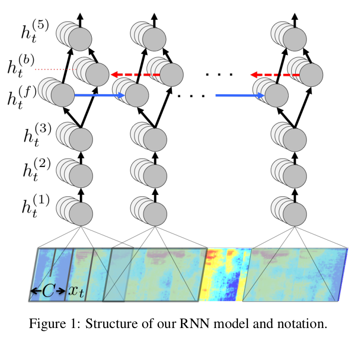
A single layer RNN was sandwiched between three 1D Convolutions and one fully connected layer and trained on the speech spectrograms. The fully connected layers used a clipped ReLu activation function. The fourth layer or the first RNN layer was bidirectional and the final layer took both forward and backward representations as input and used a softmax activation after. The model was expected to take as input the frequency bin information in time series and output the probabilities of different characters given the previous input and previous characters.

They also used some basic data augmentation methods like translating the spectrogram in time (5 ms). For regularization, a dropout of 5-10% was used on the non-recurrent layers.

Language Model

For decoding with the speech RNN, they use a language model that helps in rectifying the spelling errors which are correct phonetically, but not in line with the language spellings and grammar. The language model used is an n-gram based model which was trained using the KemLM toolkit.

The combined objective of the model is to find a sequence that will maximize the following

$Q(c) = log(P(c | x)) + \alpha log(P_{lm}(c)) + \beta * word\_count(c)$

where $\alpha$ and $\beta$ are tunable parameters that control the trade-off between the RNN, the language model, and the length of the sentence.

A beam decoder with a typical beam size in the range of $1000-8000$ is used.

Data and Model Parallelism

To increase the efficiency of the models during training and inference, different mechanisms of parallelism are used. Data is split across multiple GPUs computing gradients for mini-batches that are created by clubbing together samples of similar lengths and padding with silences. The gradient updates are calculated the usual way which is by adding up the gradients across the parallel tasks.

Data Parallelism yields speedups in training, but faces a tradeoff as larger mini-batch sizes fail to improve the training convergence rate. Another way to scale up is by parallelizing the model. This is done trivially by splitting the model across time for the non-recurrent layers. One half of the sequence is assigned to one GPU and the second to another.

For recurrent layers, the first GPU computes for the first half, the forward activations whereas the second GPU computes the backward activations. The two then swap roles, exchange the intermediate activations and finish up the forward and backward computations.  

Strided RNN

Finally, another optimization made to scale up the training and inference is to use an RNN that takes steps of size 2, making the unrolled RNN half the size of the original unstrided RNN.

DeepSpeech2

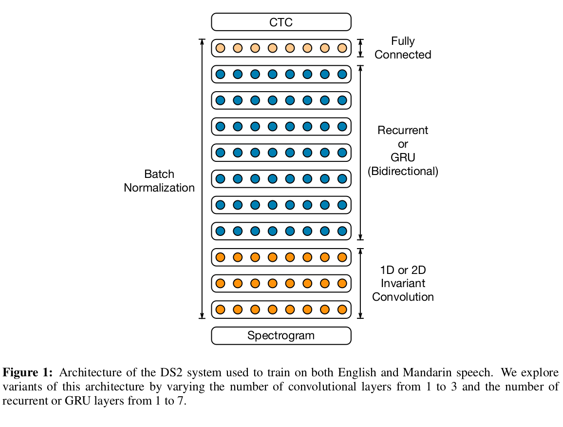
Deep Speech 2 demonstrates the performance of end-to-end ASR models in English and Mandarin, two very different languages. Apart from experimenting with model architectures, a good chunk of the work in this paper is directed toward increasing the performance of the deep learning models using HPC (High-Performance Computing) techniques that made it possible to run training experiments within days instead of weeks. They also show that by using a technique called Batch Dispatch on GPUs in a data center, the models can be in an inexpensive manner deployed for low latency online ASR.

The model used for this is deeper than the DeepSpeech model. There are several bidirectional recurrent layers used along with batch normalization. CTC loss is used as the loss function to align the speech emissions with textual predictions. The recurrent layers were also replaced by GRUs in some experiments. GRU architectures achieved better WER (word error rate) for all network depths.

Batch Normalization

The batch normalization across the layers was able to improve the final generalization error while accelerating training. Batch normalization for recurrent networks is a little tricky and in the paper, they mention that sequence-wise normalization was able to rectify issues that came up while using step-wise normalization and accumulating an average over successive time-steps, both approaches leading to no improvements in optimization while increasing the complexity of backpropagation.

BatchNorm works well in training but becomes difficult to implement in a deployed online ASR system due to the need to evaluate every utterance rather than a batch. They store a running average of the mean and variance for each neuron collected during training and use these in the inference deployment.

SortaGrad

Longer sequences usually contribute more to the cost function (CTC in this case) and are used as a heuristic for the difficulty of the utterance. The data then is sorted by utterance length and the mini-batches are created accordingly for the first epoch. For the epochs following that, random sampling of mini-batches is used. The authors dub this approach "SortaGrad". This kind of curriculum strategy improves the model performance as the model gets deeper. The effect is more pronounced when used along with BatchNorm.

This approach's effectiveness could be attributed to the fact that we often use the same learning rate even when the difference in the sequence sizes amounts to substantial differences in gradient values.

Frequency Convolutions

Temporal Convolutions are used in DeepSpeech as well as DeepSpeech 2. In DeepSpeech 2, the features used are in time as well as frequency domain. DeepSpeech 1 used spectrograms as inputs and a temporal convolution as the first layer. DeepSpeech 2 experiments with one and three such convolutional layers. They apply convolution in the `same` mode allowing them to preserve the input features in frequency as well as time. They find that 1D-invariant convolutions do not provide much benefit on cleaned or noisy data. 2D invariant convolutions improve results substantially on noisy data and marginally on cleaned data.

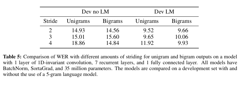
The striding for these convolutions was not done in a straightforward way as that didn't produce great results. Instead, they use non-overlapping bi-grams as their labels instead of words that are larger in number and account for several larger time steps. For example, The sentence "the cat sat" with non-overlapping bigrams is segmented as $[th, e, space, ca, t, space, sa, t]$. Notice that the last word for odd-numbered words becomes a unigram. A Space is also considered a unigram. The results are shown below.

Row Convolutions

They design a special layer in order to remove the bi-directionality in the RNNs used in DeepSpeech 1. They use the future context of a particular time step and calculate the activations based on the feature matrix $h_{t:t + \tau} = [h_t, h_{t+1}, ... ,h_{t + \tau}]$ of size $ d x (\tau + 1)$ and a parameter matrix W of the same size. $\tau$ here represents the time steps in the future context.

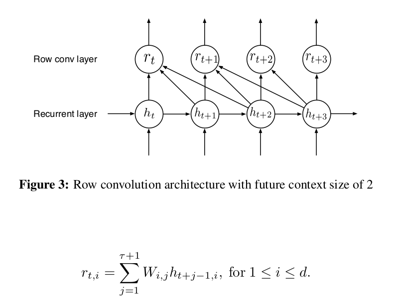
Due to the convolution-like operation shown above, they call this a Row Convolution.

Wav2Letter

The authors of this paper use three different kinds of input features: MFCCs, power-spectrum, and raw waveform.  The output of this model is one score per letter, given a dictionary $L$. They use standard 1D Convolutional Networks for acoustic modeling. Except for the first two layers where strided convolutions are used in order to make the training more efficient. The idea is that the input sequences can be long and the first layer of convolution if strided can reduce the compute required for all the layers following it. A 4-gram language model and a beam decoder are used for the final transcription.

Auto Segmentation Criterion (CTC alternative)

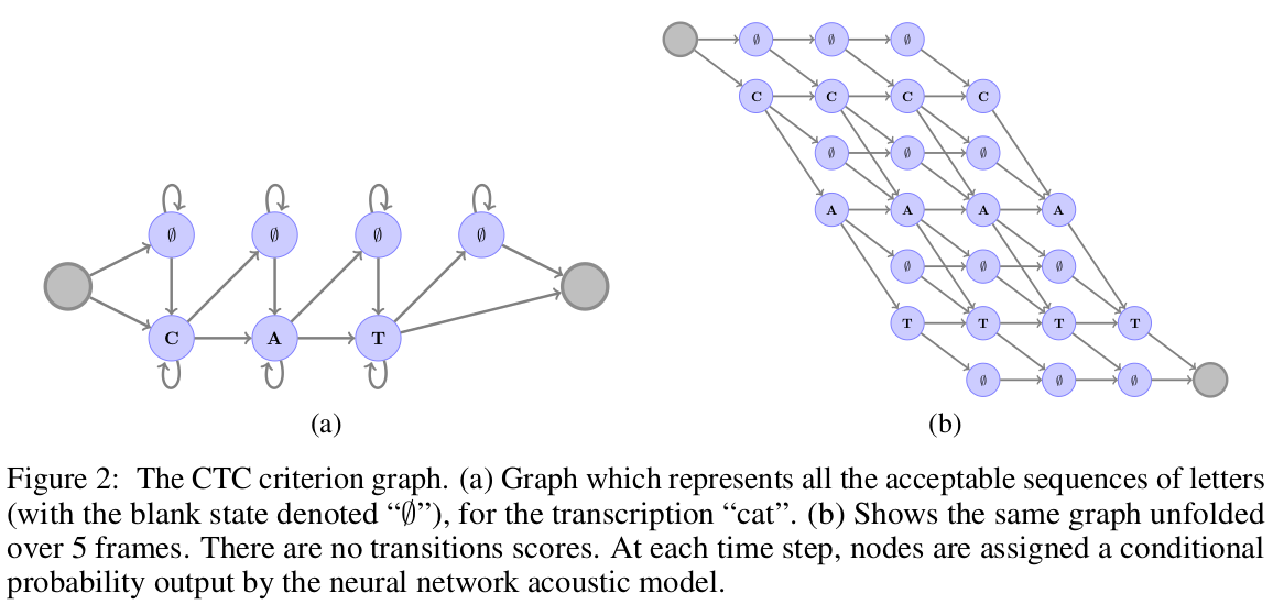
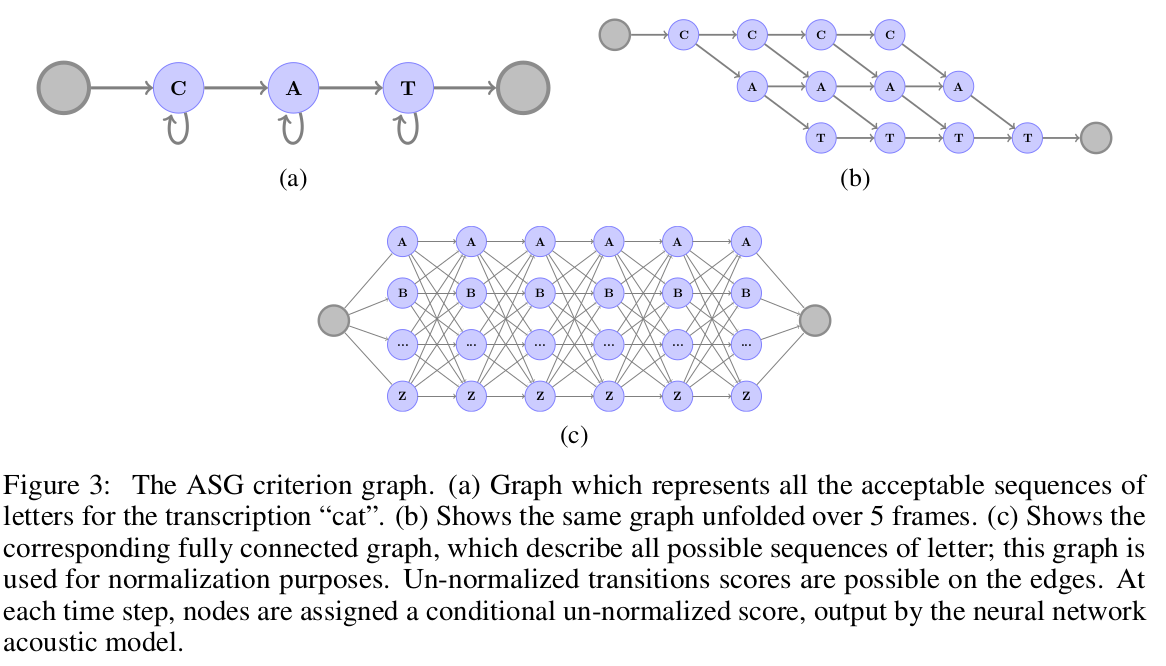
The main contribution in this paper is the alternative loss they use called the Auto Segmentation Criterion. It is different from the popular CTC Loss in the following ways:

1. There are no blank labels. They found that the blank label plays no role in modeling "garbage" frames. As for modeling repetition in letters, they use a different way to encode these with extra labels. For example $caterpillar$ becomes $caterpil2ar$.  
2. Un-normalized scores at all the nodes in the CTC criterion graph. This makes plugging different language scores much more straightforward.
3. Global normalization instead of per-frame normalization.

Jasper

Jasper uses only 1D convolutions (similar to Wav2Letter), batch normalization, ReLu, dropout, and residual connections in the model. They also propose a layer-wise optimizer called NovoGrad.  

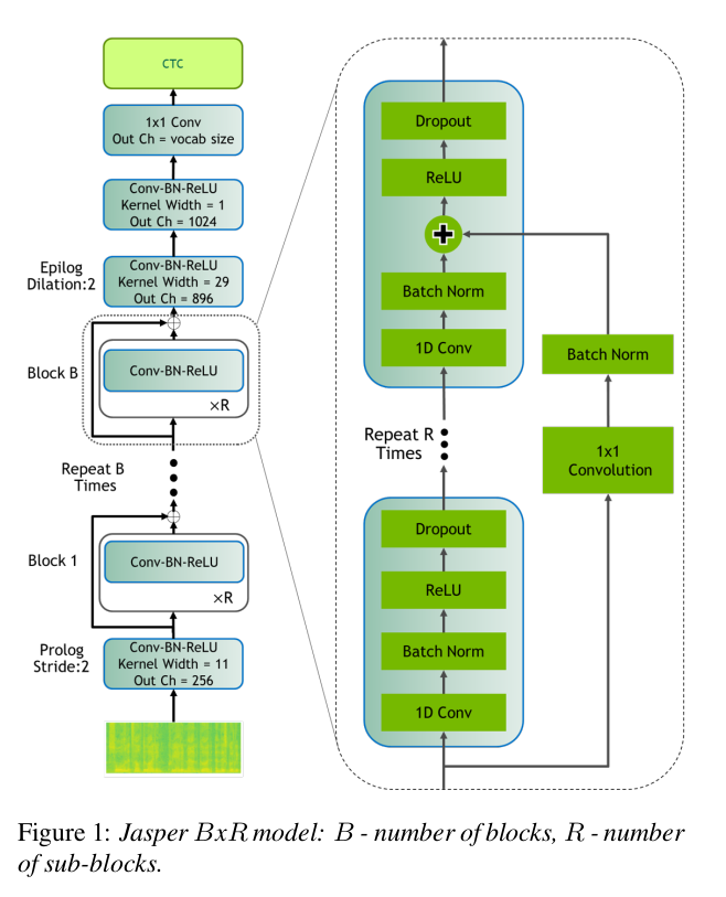
The paper explains the architecture as follows:

"Jasper uses MFCCs calculated from 20ms windows with a 10ms overlap and outputs a probability distribution over characters per frame. Jasper has a block architecture: a Jasper BxR model has B blocks, each with R sub-blocks. Each sub-block applies the following operations: a 1D-convolution, batch norm, ReLU, and dropout. All sub-blocks in a block have the same number of output channels."

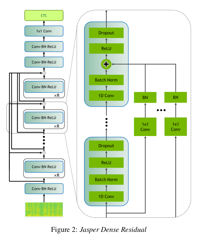
They also built a Jasper variant that instead of having connections within a block, has connections across blocks. The output of each convolutional block is added to the input of all the following convolutional blocks. They call this Jasper DR or Jasper Dense Residual model.

NovoGrad

NovoGrad is similar to the Adam Optimizer which computes adaptive learning rates for each optimization step by looking at first and second moments calculated from gradients and a constant parameter. Part of it is similar to momentum, but Adam performs better in cases where the velocity for momentum-based optimization is high, as it provides an opposing force for gradient steps in terms of the second moment.

In NovoGrad, its second moments are calculated per layer instead of per weight. This reduces memory consumption and is found to be more numerically stable by the authors. At each step, NovoGrad computes the stochastic gradients normally. The second order moment is computed for each layer as follows:

$ v ^ {l}_{t} = \beta_{2} . v ^ {l}_{t-1} + {1 - \beta_{2}} .  || g ^{l}_{t} || ^ {2}$

The second order moment is used to re-scale gradients $g_{t}^{l}$ before the calculation of the first order moment. L2-regularization is used, and a weight decay is added to the re-scaled gradient.

$ m^{l}_{t} = \beta_{1} . m ^ {l}_{t - 1} + \frac {g ^ {l}_{t}}{\sqrt {v ^ {l}_{t} + \epsilon}}  + d . w_{t}$

Wav2Vec

Wav2Vec explores unsupervised pre-training for speech recognition. They use raw audio as input and train on large amounts of data using a contrastive loss. They use these representations to fine-tune supervised task models and find their performance on par with the state of the art. The model used is a simple multi-layer convolutional layer trained for the next time-step prediction task.

Encoder network + Context Network

They apply two networks to the raw audio signal input. An encoder network embeds the audio signal in a latent space and the context network combines multiple time-steps of the encoder to obtain contextualized representations. The encoder network is a five-layer convolutional network. The output of the encoder is a low-frequency representation. The context network on the other hand has 9 layers and mixes multiple latent representations into a single context tensor. It takes the output of the encoder network as the input.

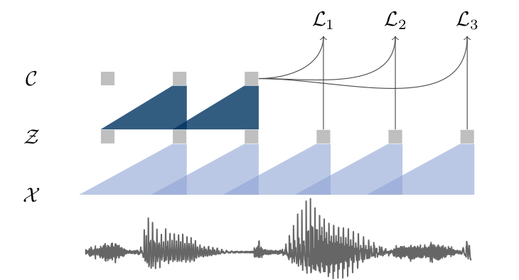
Each layer in both encoder and context networks includes a Causal Convolution with 512 channels,  a normalization layer, and a ReLu activation. The normalization is done across the time and feature dimensions to avoid variation due to scaling and input offset. For a larger model, the authors found it important to introduce residual connections in the encoder and context networks. A fully connected layer is applied at the end of the context network to produce the context embeddings.

Contrastive Loss

A contrastive loss is used to compare the similarity between the distractor samples (created through a prior distribution applied on the input till the required time step) and the sigmoid of the context embeddings. The loss is found by comparing the distractor samples from time $t$ till time $t + k$ with the sigmoid of the context embedding.

They test these embeddings across several datasets by replacing the MFCC representations. Decoding is done using a 4-gram KenLM language model and a beam decoder. The optimizer used is Adam along with a cosine learning rate schedule.

Wav2Vec 2.0

This work builds on the Wav2Vec model by adding a masked transformer on top of the stacked CNNs, a quantized form of the CNN representations and the contrastive loss takes into consideration the transformer output for time step $ T $ and quantized representations of the CNN from $ t = 1 .... T $.

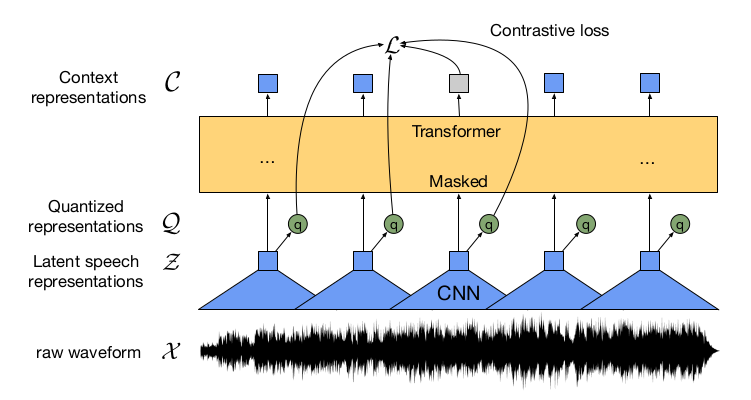
The model is trained on a large amount of unlabelled data by masking the inputs at different time steps, similar to Wav2Vec, and then trained for supervised tasks for comparison with other methods and frameworks.

Feature Encoder

The encoder consists of several temporal convolutions + layer normalization + GELU activation blocks. The representations generated from the convolutional encoder are passed on to a context network that follows the Transformer architecture. The fixed positional embedding from transformer architecture is replaced by another convolutional layer that acts like a relative positional embedding.

Quantization Module

Product Quantization is used to quantize the representations coming from the convolutional encoder. Product quantization involves splitting each vector into subspaces, and finding the centroid of each of the subspaces using k-means clustering, these centroids represent a codebook. Once the clustering model is trained, every vector is mapped to its nearest centroid from the codebook for each subspace. Each centroid for each subspace is converted to a symbolic code (hence the name codebook) that consumes much less memory. The concatenated version of these final vectors is our product quantized representation. Gumbel Softmax is used to map the output of the feature encoder to logits.

Contrastive Loss

The total optimization objective is something as follows:

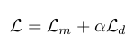
where$  L_m $ is the contrastive loss which on a backward pass would train the model to identify true quantized latent speech representation from the $ K $ distractor samples.

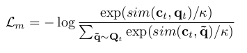
where $ c_t $ is context vector, $ q_t $ is the quantized representation and $ q $  is the set of distractors and $ q_t $.

Diversity Loss

The diversity loss is designed to increase the use of the quantized codebook representations. This is done by maximizing the entropy of the averaged softmax distribution $ l $ over the codebook entries for each codebook across a batch of utterances.

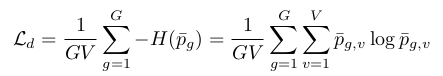
where $ G $ is the number of codebooks,$ V $ are the entries in each codebook, $ p_g $ represents each codebook, $ p_{g, v} $ is the $ v^{th} $ entry in $ p_g $.

ContextNet

ContextNet goes beyond the CNN-RNN-Transducer architectures and experiments with fully convolutional layers with squeeze-and-excitation modules. They also introduce a simple network scaling method that provides a good result on the accuracy vs compute tradeoff. The authors argue that the lack of global context obtained by CNN-based architectures due to limited kernel size is the main reason for their lower performance when compared to transformer-based or RNN-based models, given that the latter technically have access to the entire sequence for modeling.

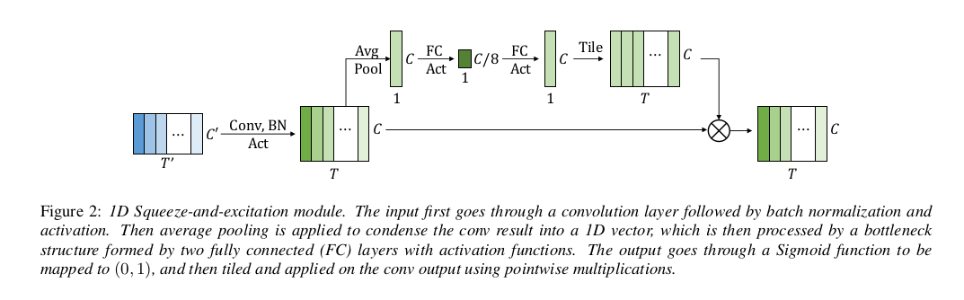
Squeeze And Excitation Networks

To solve for the inability of CNNs to generalize over a longer context in a given sequence, they introduce Squeeze and Excitation modules in their convolutional architectures. Squeeze and Excitation modules work by encoding a multi-channel, multi-feature input into a single neuron per channel. This representation is encoded by a fully connected layer (the squeezing) to a smaller representation reduced by a factor $r$, hence reducing the number of neurons to $ C / r $. These neurons are then passed through another fully connected layer (the excitation) to broadcast the compressed representation back to the size of the original global context vector.

The authors use RNN-T decoding instead of a CTC decoder. They also use the swish activation function which adds to minor but consistent reductions in the WER.  

Another contribution of this paper is the scaling scheme that downsamples the input progressively by globally changing the number of channels in various convolutional layers. This reduces model size significantly while maintaining good accuracy.

Emformer

This paper gets its name from "Efficient Memory transFORMER" as they optimize the transformer architecture in order to serve low latency streaming speech recognition applications. This paper builds on top of the AM-TRF method.  

AM-TRF

AM-TRF or the "Augmented Memory Transformer" limits the left context length of the input, breaks the input sequence into chunks for the transformer to parallelize, and uses a memory bank to capture long-range dependencies that self-attention in each block would not be able to capture.

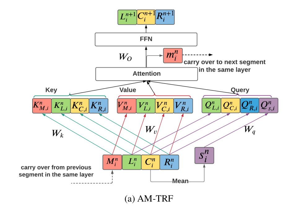
The input is broken into $I$ non-overlapping segments $C_{1} ^ {n} ... C_{I - 1} ^ {n}$. Assume $n$ to be the layer index. Each of these input chunks are, to avoid boundary effects, concatenated with the left and right contextual blocks $L_{i}^{n} $ and $ R_{i} ^ {n}$ to form the contextual segment $X_{i} ^ {n}$. The AM-TRF layer takes a memory bank $ M_{i} ^ {n} = [m_{1} ^ {n} ... m_{i - 1} ^ {n}]$ and $ X_{i} ^ {n}$ as input and output $ X_{i + 1} ^ {n}$ and memory vector $m_{i} ^ {n}$.

Caching Keys and Values

The authors recognize that AM-TRF has performed well on streaming speech recognition tasks but its architecture has some drawbacks. For example, it does not use the Left Context efficiently. As shown in the figure above, the left context vector has to be recomputed every time, even though they might overlap with the center context.

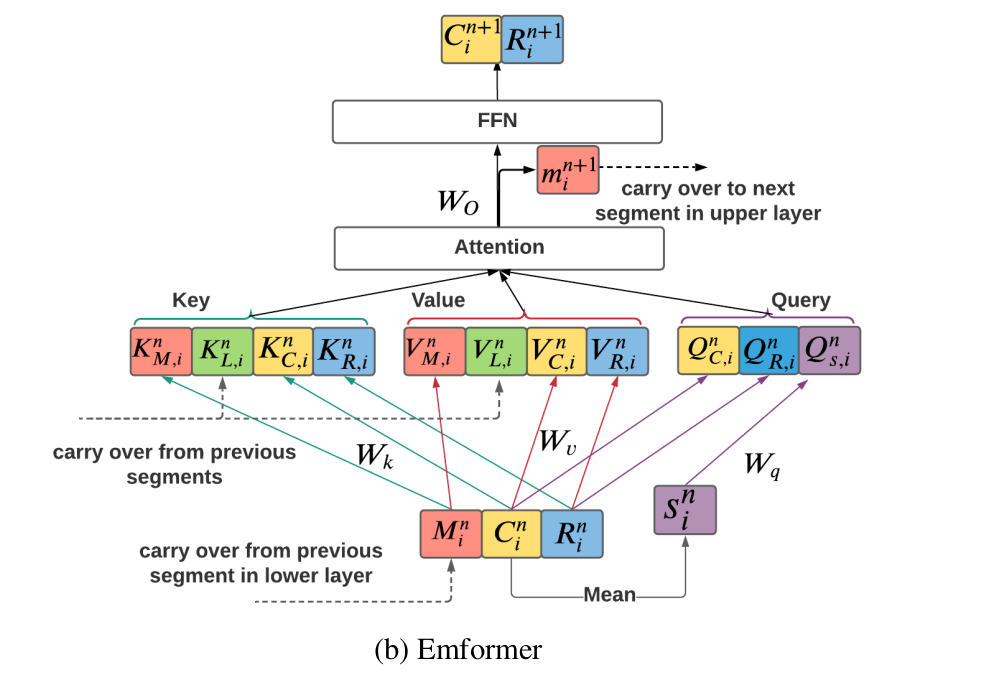
They propose a key value caching mechanism for the left context that can be carried over from previous segments, reducing the compute substantially.

Memory Carry Over

The block processing mechanism in AM-TRF requires every time step to have the memory bank from the previous time step as an input for the same layer. This limits the GPU parallelization and usage. To allow faster compute, Emformer passes the memory vector output from the attention mechanism to the next segment of the next layer instead of the same layer's next block.

Right Context Leak

Also, to avoid look-ahead context leaking, the Emformer model uses a masking mechanism during training which is in contrast with the AM-TRF model which uses sequential block processing.

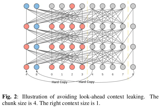
"Emformer makes a hard copy of each segment’s look-ahead context and puts the look-ahead context copy at the input sequence’s beginning. For example, the output at frame 2 in the first chunk only uses the information from the current chunk together with the right context frame 4 without the right context leaking."

Conformer

Conformer or the "CONvolution-augmented TransFORMER" merges the best of both worlds - the local feature learning of the convolutions and the global context learning of the recurrent networks and transformers in a parameter-efficient manner.  

Conformer Encoder

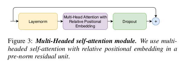
A conformer block has four components to it, namely, a feed-forward module, a self-attention module, a convolution module, and a second feed-forward module in the end.

For the self-attention module, they take inspiration from the Transformer-XL paper and their relative sinusoidal positional encoding scheme. This helps the model generalize over varying sequence lengths better.

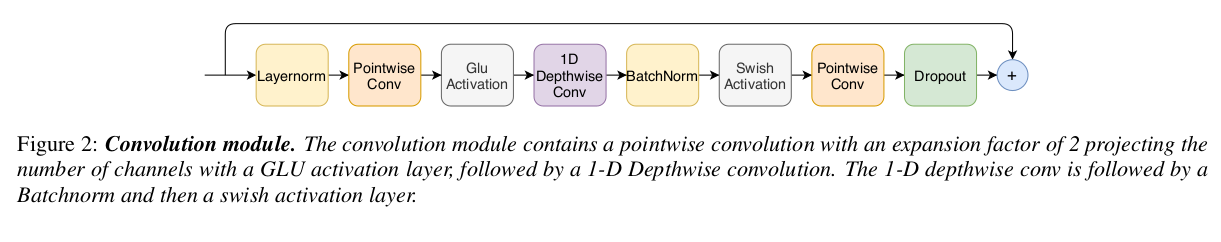
The convolution module uses a pointwise convolution with GLU activation, a 1D depthwise convolution, batch normalization with a swish activation, and ends with another pointwise convolution and dropout.

The feed-forward modules consist of two linear transformations and a non-linear transformation (swish activation) in between.

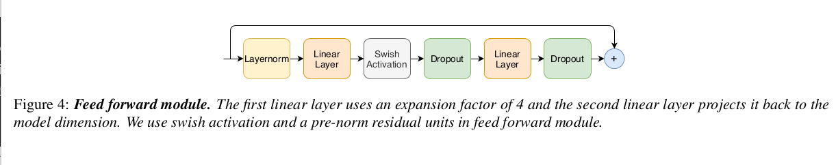
The proposed conformer block sandwiches the multi-headed self-attention block and the convolution block between two feed-forward blocks.

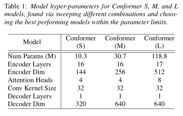
A single-layer LSTM decoder is used as the decoder for all their experiments. They sweep through several architectural hyperparameters for three different model sizes - 10M, 30M, and 118M parameters.

Conclusion

We have been looking into audio data in the last few articles. We looked at audio processing, and music analysis, and in the previous article explored the basics of the automatic speech recognition problem. In this article, we explored the ways people have employed deep learning to solve the problem of ASR end-to-end using temporal convolutions, recurrent networks, transformer architectures, variations of each of these, hybrids of more than one of these, etc. We have also looked at some of the ways the problem was looked at in terms of compute required by compressing networks using quantization, modifying model architectures, and parallelizing them in order to make them more efficient.

In the coming articles, we will look at end-to-end frameworks available open-source and also implement a training and prediction pipeline using the Conformer architecture.