Attention - "notice taken of someone or something"
Modern day techniques employed in Neural Networks in the domain of Computer Vision include "Attention Mechanisms". Computer Vision has aimed to emulate human visual perception in terms of code-based algorithms. Before diving further into the Attention Mechanisms used in Computer Vision, let's take a brief look at how attention mechanisms are embedded in and inspired by human visual capabilities.
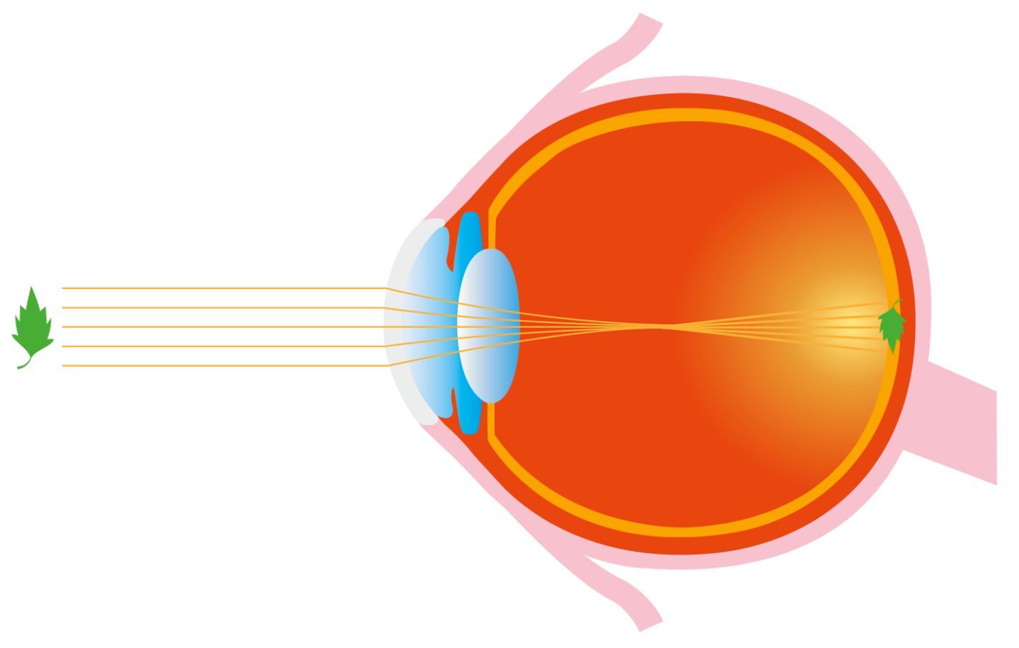
In the diagram above, the light traverses from the object of interest (which in this case is a leaf) to the Macula, which is the primary functional region of the Retina inside the eye. However, what happens when we have multiple objects in the field of view?
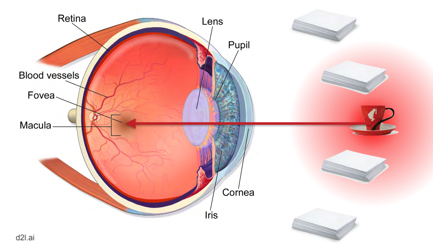
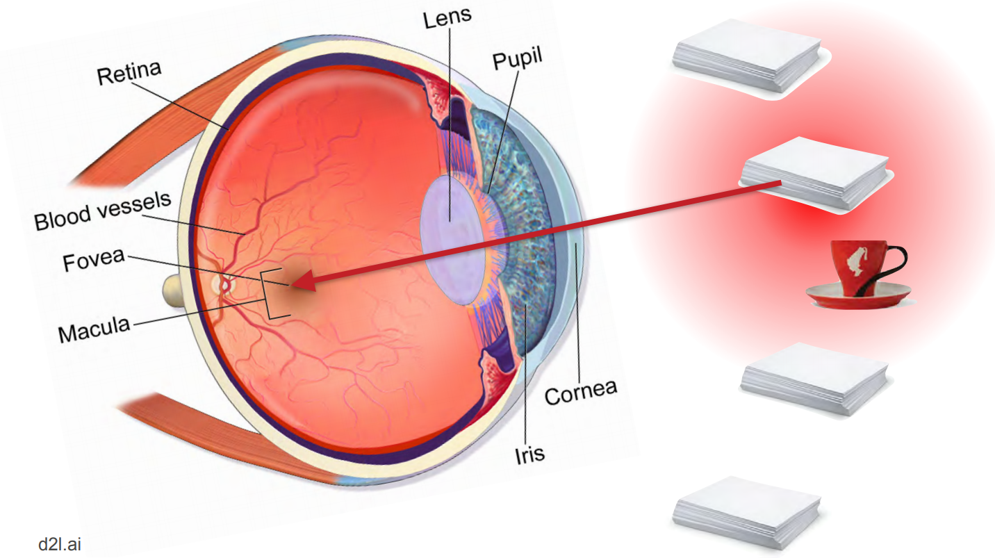
When we must focus on a single object when there is an array of diverse objects in our field of view, the attention mechanism within our visual perception system uses a sophisticated group of filters to create a blurring effect (similar to that of "Bokeh" in digital photography) so the object of interest is in focus, while the surrounding is faded or blurred.
Now, back to Attention Mechanisms in Deep Learning. The idea of Attention Mechanisms was first popularly introduced in the domain of Natural Language Processing (NLP) in the NeurIPS 2017 paper by Google Brain, titled "Attention Is All You Need".
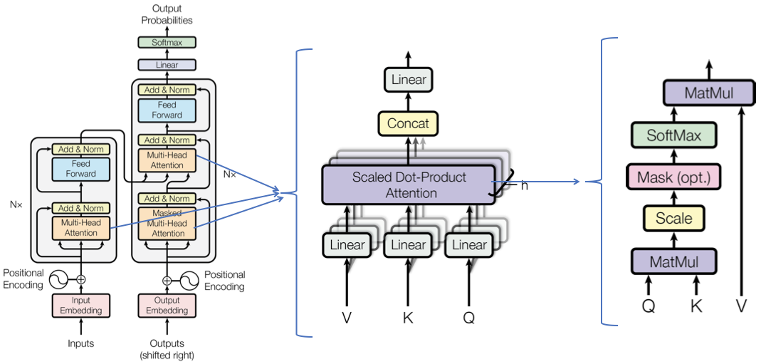
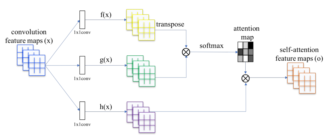
In this paper the attention mechanism was computed using three main components: Query, Key, and Value. We will go through these concepts in an upcoming post, however, this idea was first ported into Computer Vision in the Self Attention Generative Adversarial Networks paper (also popularly known by its abbreviation, SAGAN). This paper introduced the Self Attention Module as shown in the following diagram (f(x), g(x), and h(x) represent query, key and value, respectively):
In this post we'll discuss a different form of attention mechanism in Computer Vision, known as the Convolutional Block Attention Module (CBAM).
Table of Contents:
- Convolutional Block Attention Module (CBAM):
- What are Spatial Attention and Channel Attention?
a. So, what's meant by Spatial Attention?
b. Then what's Channel Attention, and do we even need it?
c. Why use both, isn't either one sufficient? - Spatial Attention Module (SAM)
- Channel Attention Module (CAM)
a. So what is the difference between Squeeze Excitation Module and Channel Attention Module? - In Conclusion
- Ablation study and results
- What are Spatial Attention and Channel Attention?
- References
Bring this project to life
Convolutional Block Attention Module (CBAM)
Although the Convolutional Block Attention Module (CBAM) was brought into fashion in the ECCV 2018 paper titled "CBAM: Convolutional Block Attention Module", the general concept was introduced in the 2016 paper titled "SCA-CNN: Spatial and Channel-wise Attention in Convolutional Networks for Image Captioning". SCA-CNN demonstrated the potential of using multi-layered attention: Spatial Attention and Channel Attention combined, which are the two building blocks of CBAM in Image Captioning. The CBAM paper was the first to successfully showcase the wide applicability of the module, especially for Image Classification and Object Detection tasks.
Before diving into the details of CBAM, let's take a look at the general structure of the module:
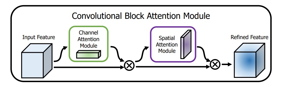
CBAM contains two sequential sub-modules called the Channel Attention Module (CAM) and the Spatial Attention Module (SAM), which are applied in that particular order. The authors of the paper point out that CBAM is applied at every convolutional block in deep networks to get subsequent "Refined Feature Maps" from the "Input Intermediate Feature Maps".
What are Spatial Attention and Channel Attention?
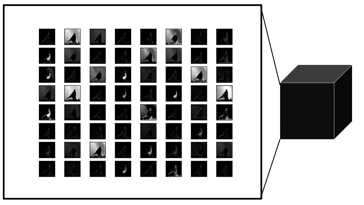
The words Spatial and Channel are probably the most referred-to terms in Computer Vision, especially when it comes to convolutional layers. In any convolutional layer the input is a tensor and the subsequent output is a tensor. This tensor is characterized by 3-dimensional metrics: h for the height of each feature map; w for the width of each feature map; and c for the total number of channels, the total number of feature maps, or the depth of the tensor. This is why we usually denote the dimensions of the input as (c × h × w). The feature maps are essentially each slice of the cube-shaped tensor shown below, i.e., the feature maps are stacked together. The c dimension value is decided by the total number of convolution filters used in that layer. Before going through the specifics of Spatial and Channel Attention respectively, let's get to know what these terms mean and why they are essential.
So, what's meant by Spatial Attention?
Spatial refers to the domain space encapsulated within each feature map. Spatial attention represents the attention mechanism/attention mask on the feature map, or a single cross-sectional slice of the tensor. For instance, in the image below the object of interest is a bird, thus the Spatial Attention will generate a mask which will enhance the features that define that bird. By thus refining the feature maps using Spatial Attention, we are enhancing the input to the subsequent convolutional layers which thus improves the performance of the model.
Then what's channel attention, and do we even need it?
As discussed above, channels are essentially the feature maps stacked in a tensor, where each cross-sectional slice is basically a feature map of dimension (h x w). Usually in convolutional layers, the trainable weights making up the filters learn generally small values (close to zero), thus we observe similar feature maps with many appearing to be copies of one another. This observation was a main driver for the CVPR 2020 paper titled "GhostNet: More Features from Cheap Operations". Even though they look similar, these filters are extremely useful in learning different types of features. While some are specific for learning horizontal and vertical edges, others are more general and learn a particular texture in the image. The channel attention essentially provides a weight for each channel and thus enhances those particular channels which are most contributing towards learning and thus boosts the overall model performance.
Why use both, isn't either one sufficient?
Well, technically yes and no; the authors in their code implementation provide the option to only use Channel Attention and switch off the Spatial Attention. However, for best results it has been advised to use both. In layman terms, channel attention says which feature map is important for learning and enhances, or as the authors say, "refines" it. Meanwhile, the spatial attention conveys what within the feature map is essential to learn. Combining both robustly enhances the Feature Maps and thus justifies the significant improvement in model performance.
Spatial Attention Module (SAM)
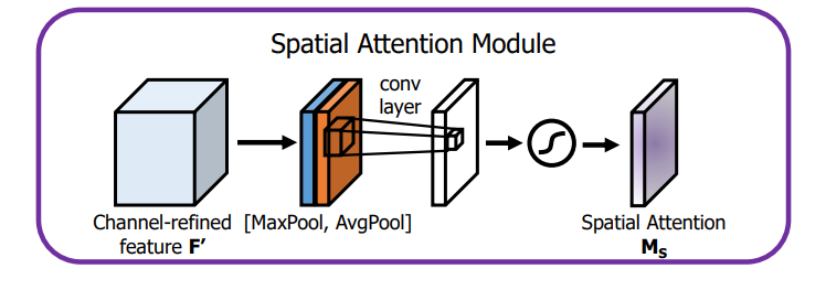
Spatial Attention Module (SAM) is comprised of a three-fold sequential operation. The first part of it is called the Channel Pool, where the Input Tensor of dimensions (c × h × w) is decomposed to 2 channels, i.e. (2 × h × w), where each of the 2 channels represent Max Pooling and Average Pooling across the channels. This serves as the input to the convolution layer which output a 1-channel feature map, i.e., the dimension of the output is (1 × h × w). Thus, this convolution layer is a spatial dimension preserving convolution and uses padding to do the same. In code, the convolution is followed by a Batch Norm layer to normalize and scale the output of convolution. However, the authors have also provided an option to use ReLU activation function after the Convolution layer, but by default it only uses Convolution + Batch Norm. The output is then passed to a Sigmoid Activation layer. Sigmoid, being a probabilistic activation, will map all the values to a range between 0 and 1. This Spatial Attention mask is then applied to all the feature maps in the input tensor using a simple element-wise product.
The authors validated different approaches of computing Spatial Attention using SAM in the ImageNet classification task. The results from the paper are shown below:
| Architecture | Parameters (in millions) | GFLOPs | Top-1 Error (%) | Top-5 Error (%) |
|---|---|---|---|---|
| Vanilla ResNet-50 | 25.56 | 3.86 | 24.56 | 7.5 |
| ResNet-50 + CBAM1 | 28.09 | 3.862 | 22.8 | 6.52 |
| ResNet-50 + CBAM (1 x 1 conv, k = 3)2 | 28.10 | 3.869 | 22.96 | 6.64 |
| ResNet-50 + CBAM (1 x 1 conv, k = 7)2 | 28.10 | 3.869 | 22.9 | 6.47 |
| ResNet-50 + CBAM (AvgPool + MaxPool, k = 3)2 | 28.09 | 3.863 | 22.68 | 6.41 |
| ResNet-50 + CBAM (AvgPool + MaxPool, k = 7)2 | 28.09 | 3.864 | 22.66 | 6.31 |
1 - CBAM here represents only the Channel Attention Module (CAM), Spatial Attention Module (SAM) was switched off.
2 - CBAM here represents both CAM + SAM. The specifications within the brackets show the way of computing the Channel Pool and the kernel size used for the convolution layer in SAM.
PyTorch code implementation of the Spatial Attention components:
import torch
import torch.nn as nn

class BasicConv(nn.Module):
    def __init__(self, in_planes, out_planes, kernel_size, stride=1, padding=0, dilation=1, groups=1, relu=True, bn=True, bias=False):
        super(BasicConv, self).__init__()
        self.out_channels = out_planes
        self.conv = nn.Conv2d(in_planes, out_planes, kernel_size=kernel_size, stride=stride, padding=padding, dilation=dilation, groups=groups, bias=bias)
        self.bn = nn.BatchNorm2d(out_planes,eps=1e-5, momentum=0.01, affine=True) if bn else None
        self.relu = nn.ReLU() if relu else None

    def forward(self, x):
        x = self.conv(x)
        if self.bn is not None:
            x = self.bn(x)
        if self.relu is not None:
            x = self.relu(x)
        return x

class ChannelPool(nn.Module):
    def forward(self, x):
        return torch.cat( (torch.max(x,1)[0].unsqueeze(1), torch.mean(x,1).unsqueeze(1)), dim=1 )

class SpatialGate(nn.Module):
    def __init__(self):
        super(SpatialGate, self).__init__()
        kernel_size = 7
        self.compress = ChannelPool()
        self.spatial = BasicConv(2, 1, kernel_size, stride=1, padding=(kernel_size-1) // 2, relu=False)
    def forward(self, x):
        x_compress = self.compress(x)
        x_out = self.spatial(x_compress)
        scale = F.sigmoid(x_out) # broadcasting
return x * scaleChannel Attention Module (CAM)
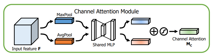
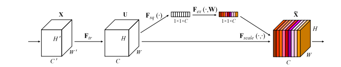
The Channel Attention Module (CAM) is another sequential operation but a bit more complex than Spatial Attention Module (SAM). At first glance, CAM resembles Squeeze Excite (SE) layer. Squeeze Excite was first proposed in the CVPR/ TPAMI 2018 paper titled: 'Squeeze-and-Excitation Networks'. To briefly recap, this is how the SE block looks:
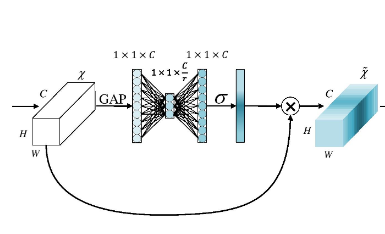
To more concisely interpret a SE-block, the following diagram of SE-block from the CVPR-2020 paper titled "ECA-Net: Efficient Channel Attention for Deep Convolutional Neural Networks" shows the clear similarity between a Squeeze Excitation block and the Channel Attention Module in the Convolutional Block Attention Module (note: we will cover ECANet in an upcoming post in this series).
So what's the difference between Squeeze Excitation and Channel Attention Module?
Before answering that, let's do a quick review of the Squeeze Excitation Module. The Squeeze Excitation Module has the following components: Global Average Pooling (GAP), and a Multi-layer Perceptron (MLP) network mapped by reduction ratio (r) and sigmoid activation. The input to the SE block is essentially a tensor of dimension (c × h × w). Global Average Pooling is essentially an Average Pooling operation where each feature map is reduced to a single pixel, thus each channel is now decomposed to a (1 × 1) spatial dimension. Thus the output dimension of the GAP is basically a 1-D vector of length c which can be represented as (c × 1 × 1). This vector is then passed as the input to the Multi-layer perceptron (MLP) network which has a bottleneck whose width or number of neurons is decided by the reduction ratio (r). The higher the reduction ratio, the fewer the number of neurons in the bottleneck and vice versa. The output vector from this MLP is then passed to a sigmoid activation layer which then maps the values in the vector within the range of 0 and 1.
Channel Attention Module (CAM) is pretty similar to the Squeeze Excitation layer with a small modification. Instead of reducing the Feature Maps to a single pixel by Global Average Pooling (GAP), it decomposes the input tensor into 2 subsequent vectors of dimensionality (c × 1 × 1). One of these vectors is generated by GAP while the other vector is generated by Global Max Pooling (GMP). Average pooling is mainly used for aggregating spatial information, whereas max pooling preserves much richer contextual information in the form of edges of the object within the image which thus leads to finer channel attention. Simply put, average pooling has a smoothing effect while max pooling has a much sharper effect, but preserves natural edges of the objects more precisely. The authors validate this in their experiments where they show that using both Global Average Pooling and Global Max Pooling gives better results than using just GAP as in the case of Squeeze Excitation Networks.
The following table shows some results on ImageNet classification from the paper validating the use of GAP + GMP:
| Architecture | Parameters (in millions) | GFLOPs | Top-1 Error (%) | Top-5 Error (%) |
|---|---|---|---|---|
| Vanilla ResNet-50 | 25.56 | 3.86 | 24.56 | 7.5 |
| SE-ResNet-50 (GAP) | 25.92 | 3.94 | 23.14 | 6.7 |
| ResNet-50 + CBAM1 (GMP) | 25.92 | 3.94 | 23.2 | 6.83 |
| ResNet-50 + CBAM1 (GMP + GAP) | 25.92 | 4.02 | 22.8 | 6.52 |
1 - CBAM here represents only the Channel Attention Module (CAM), Spatial Attention Module (SAM) was switched off.
The two vectors generated by GAP and GMP are consecutively sent to the MLP network whose output vectors are subsequently summed element-wise. To note, both the inputs use the same weights for the MLP, and the ReLU activation function is used as the preferred choice for its non-linearity.
The resultant vector after being summed up is then passed to the Sigmoid activation layer, which generates the channel weights (which are simply multiplied element-wise according to each corresponding channel/feature map in the input tensor).
Here is the implementation of Channel Attention Module (CAM) in PyTorch:
import torch
import torch.nn as nn

def logsumexp_2d(tensor):
    tensor_flatten = tensor.view(tensor.size(0), tensor.size(1), -1)
    s, _ = torch.max(tensor_flatten, dim=2, keepdim=True)
    outputs = s + (tensor_flatten - s).exp().sum(dim=2, keepdim=True).log()
    return outputs

class Flatten(nn.Module):
    def forward(self, x):
        return x.view(x.size(0), -1)

class ChannelGate(nn.Module):
    def __init__(self, gate_channels, reduction_ratio=16, pool_types=['avg', 'max']):
        super(ChannelGate, self).__init__()
        self.gate_channels = gate_channels
        self.mlp = nn.Sequential(
            Flatten(),
            nn.Linear(gate_channels, gate_channels // reduction_ratio),
            nn.ReLU(),
            nn.Linear(gate_channels // reduction_ratio, gate_channels)
            )
        self.pool_types = pool_types
    def forward(self, x):
        channel_att_sum = None
        for pool_type in self.pool_types:
            if pool_type=='avg':
                avg_pool = F.avg_pool2d( x, (x.size(2), x.size(3)), stride=(x.size(2), x.size(3)))
                channel_att_raw = self.mlp( avg_pool )
            elif pool_type=='max':
                max_pool = F.max_pool2d( x, (x.size(2), x.size(3)), stride=(x.size(2), x.size(3)))
                channel_att_raw = self.mlp( max_pool )
            elif pool_type=='lp':
                lp_pool = F.lp_pool2d( x, 2, (x.size(2), x.size(3)), stride=(x.size(2), x.size(3)))
                channel_att_raw = self.mlp( lp_pool )
            elif pool_type=='lse':
                # LSE pool only
                lse_pool = logsumexp_2d(x)
                channel_att_raw = self.mlp( lse_pool )

            if channel_att_sum is None:
                channel_att_sum = channel_att_raw
            else:
                channel_att_sum = channel_att_sum + channel_att_raw

        scale = F.sigmoid( channel_att_sum ).unsqueeze(2).unsqueeze(3).expand_as(x)
return x * scaleThe authors do provide the option to use Power Average Pooling (LP-Pool) and Logarithmic Summed Exponential (LSE), which are shown in the code snippet above, however the paper doesn't discuss the results obtained when using them. For the paper, the reduction ratio (r) is set to a default value of 16.
In Conclusion
CBAM is applied as a layer in every convolutional block of a convolutional neural network model. It takes in a tensor containing the feature maps from the previous convolutional layer and first refines it by applying channel attention using CAM. Subsequently this refined tensor is passed to SAM where the spatial attention is applied, thus resulting in the output refined feature maps. The complete code for the CBAM layer in PyTorch is provided below.
import torch
import math
import torch.nn as nn

class BasicConv(nn.Module):
    def __init__(self, in_planes, out_planes, kernel_size, stride=1, padding=0, dilation=1, groups=1, relu=True, bn=True, bias=False):
        super(BasicConv, self).__init__()
        self.out_channels = out_planes
        self.conv = nn.Conv2d(in_planes, out_planes, kernel_size=kernel_size, stride=stride, padding=padding, dilation=dilation, groups=groups, bias=bias)
        self.bn = nn.BatchNorm2d(out_planes,eps=1e-5, momentum=0.01, affine=True) if bn else None
        self.relu = nn.ReLU() if relu else None

    def forward(self, x):
        x = self.conv(x)
        if self.bn is not None:
            x = self.bn(x)
        if self.relu is not None:
            x = self.relu(x)
        return x

class Flatten(nn.Module):
    def forward(self, x):
        return x.view(x.size(0), -1)

class ChannelGate(nn.Module):
    def __init__(self, gate_channels, reduction_ratio=16, pool_types=['avg', 'max']):
        super(ChannelGate, self).__init__()
        self.gate_channels = gate_channels
        self.mlp = nn.Sequential(
            Flatten(),
            nn.Linear(gate_channels, gate_channels // reduction_ratio),
            nn.ReLU(),
            nn.Linear(gate_channels // reduction_ratio, gate_channels)
            )
        self.pool_types = pool_types
    def forward(self, x):
        channel_att_sum = None
        for pool_type in self.pool_types:
            if pool_type=='avg':
                avg_pool = F.avg_pool2d( x, (x.size(2), x.size(3)), stride=(x.size(2), x.size(3)))
                channel_att_raw = self.mlp( avg_pool )
            elif pool_type=='max':
                max_pool = F.max_pool2d( x, (x.size(2), x.size(3)), stride=(x.size(2), x.size(3)))
                channel_att_raw = self.mlp( max_pool )
            elif pool_type=='lp':
                lp_pool = F.lp_pool2d( x, 2, (x.size(2), x.size(3)), stride=(x.size(2), x.size(3)))
                channel_att_raw = self.mlp( lp_pool )
            elif pool_type=='lse':
                # LSE pool only
                lse_pool = logsumexp_2d(x)
                channel_att_raw = self.mlp( lse_pool )

            if channel_att_sum is None:
                channel_att_sum = channel_att_raw
            else:
                channel_att_sum = channel_att_sum + channel_att_raw

        scale = F.sigmoid( channel_att_sum ).unsqueeze(2).unsqueeze(3).expand_as(x)
        return x * scale

def logsumexp_2d(tensor):
    tensor_flatten = tensor.view(tensor.size(0), tensor.size(1), -1)
    s, _ = torch.max(tensor_flatten, dim=2, keepdim=True)
    outputs = s + (tensor_flatten - s).exp().sum(dim=2, keepdim=True).log()
    return outputs

class ChannelPool(nn.Module):
    def forward(self, x):
        return torch.cat( (torch.max(x,1)[0].unsqueeze(1), torch.mean(x,1).unsqueeze(1)), dim=1 )

class SpatialGate(nn.Module):
    def __init__(self):
        super(SpatialGate, self).__init__()
        kernel_size = 7
        self.compress = ChannelPool()
        self.spatial = BasicConv(2, 1, kernel_size, stride=1, padding=(kernel_size-1) // 2, relu=False)
    def forward(self, x):
        x_compress = self.compress(x)
        x_out = self.spatial(x_compress)
        scale = F.sigmoid(x_out) # broadcasting
        return x * scale

class CBAM(nn.Module):
    def __init__(self, gate_channels, reduction_ratio=16, pool_types=['avg', 'max'], no_spatial=False):
        super(CBAM, self).__init__()
        self.ChannelGate = ChannelGate(gate_channels, reduction_ratio, pool_types)
        self.no_spatial=no_spatial
        if not no_spatial:
            self.SpatialGate = SpatialGate()
    def forward(self, x):
        x_out = self.ChannelGate(x)
        if not self.no_spatial:
            x_out = self.SpatialGate(x_out)
        return x_out
Ablation Study and Results
The authors validate CBAM on a huge array of experiments listing from ImageNet classification to Object Detection on MS-COCO and PASCAL VOC datasets. The authors also showcase an ablation study where they defend their idea of applying CAM and SAM in this order within CBAM, compared to the results of not applying SAM.
| Architecture | Top-1 Error (%) | Top-5 Error (%) |
|---|---|---|
| Vanilla ResNet-50 | 24.56 | 7.5 |
| SE-ResNet-50 | 23.14 | 6.7 |
| ResNet-50 + CBAM (CAM -> SAM) | 22.66 | 6.31 |
| ResNet-50 + CBAM (SAM -> CAM) | 22.78 | 6.42 |
| ResNet-50 + CBAM (SAM and CAM in parallel) | 22.95 | 6.59 |
Finally, here are the results of CBAM on ImageNet classification for some of the models presented in the paper:
| Architecture | Parameters (in millions) | GFLOPs | Top-1 Error (%) | Top-5 Error (%) |
|---|---|---|---|---|
| Vanilla ResNet-101 | 44.55 | 7.57 | 23.38 | 6.88 |
| SE-ResNet-101 | 49.33 | 7.575 | 22.35 | 6.19 |
| ResNet-101 + CBAM | 49.33 | 7.581 | 21.51 | 5.69 |
| Vanilla WideResNet18 (widen=2.0) | 45.62 | 6.696 | 25.63 | 8.20 |
| WideResNet18 (widen=2.0) + SE | 45.97 | 6.696 | 24.93 | 7.65 |
| WideResNet18 (widen=2.0) + CBAM | 45.97 | 6.697 | 24.84 | 7.63 |
| Vanilla ResNeXt50(32x4d) | 25.03 | 3.768 | 22.85 | 6.48 |
| ResNeXt50 (32x4d) + SE | 27.56 | 3.771 | 21.91 | 6.04 |
| ResNeXt50 (32x4d) + CBAM | 27.56 | 3.774 | 21.92 | 5.91 |
| Vanilla MobileNet | 4.23 | 0.569 | 31.39 | 11.51 |
| MobileNet + SE | 5.07 | 0.570 | 29.97 | 10.63 |
| MobileNet + CBAM | 5.07 | 0.576 | 29.01 | 9.99 |
And some of the noteworthy Object Detection results as shown in the paper:
MS-COCO:
| Backbone | Detector | mAP@.5 | mAP@.75 | mAP@[.5, .95] |
|---|---|---|---|---|
| Vanilla ResNet101 | Faster-RCNN | 48.4 | 30.7 | 29.1 |
| ResNet101 + CBAM | Faster-RCNN | 50.5 | 32.6 | 30.8 |
PASCAL VOC:
| Backbone | Detector | mAP@.5 | Parameters (in millions) |
|---|---|---|---|
| VGG16 | SSD | 77.8 | 26.5 |
| VGG16 | StairNet | 78.9 | 32.0 |
| VGG16 | StairNet + SE | 79.1 | 32.1 |
| VGG16 | StairNet + CBAM | 79.3 | 32.1 |
As demonstrated above, CBAM clearly outperforms the vanilla models and their subsequent squeeze excitation versions in complex networks on challenging datasets, such as ImageNet and MS-COCO.
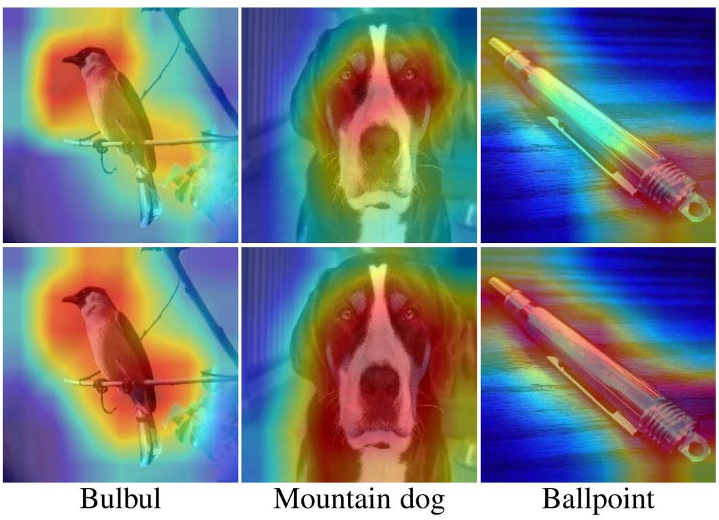
The authors even take things a step further to provide additional insight into CBAM's effect in model performance by visualizing the GradCAM results on some sample images from ImageNet, and comparing them with that of the Squeeze Excite model and the baseline vanilla model. Gradient-weighted Class Activation Maps (Grad-CAM) basically take the gradient from the final convolution layer to provide a coarse localization of the important regions within the image, which makes the model provide a prediction for that particular target label. For instance, for an image of dog, GradCAM should basically highlight the region in the image which has the dog, as that part of the image is important (or the driving reason) for the model to classify it as (i.e. recognize) a dog.
Some of the results provided by the CBAM paper are shown below:
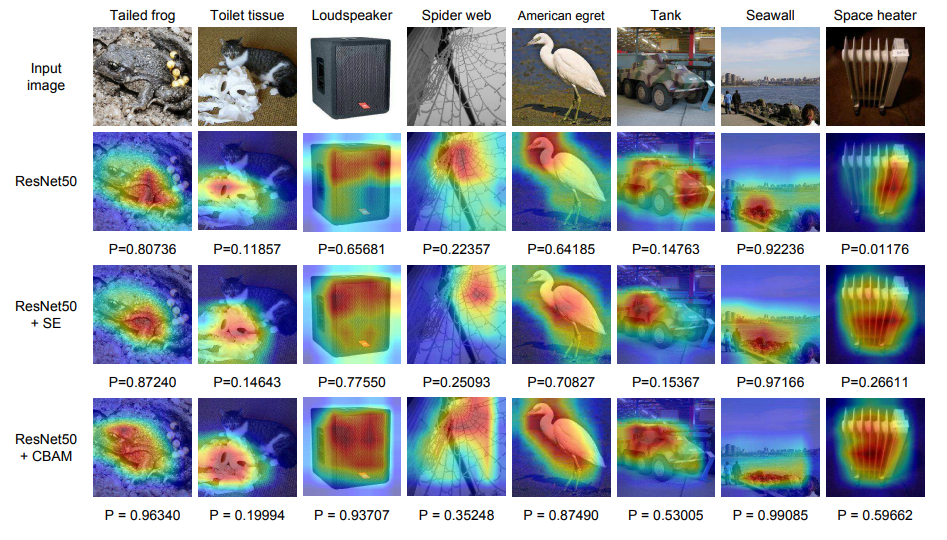
The P values at the bottom show the class confidence score, and as shown, CBAM gives much better Grad-CAM results as compared to both its SE counterpart and vanilla alike. To add icing to the cake, the authors conducted a survey where the users were shown the GradCAM results for Vanilla, SE and CBAM models of a sample of shuffled images along with their true labels, and were asked to vote on which GradCAM output highlights better contextual region depicting that label. Based on the survey, CBAM won the poll by a clear margin.
Thank you for reading.
References:
- Attention in Deep Learning, Alex Smola and Aston Zhang, Amazon Web Services (AWS), ICML 2019
- Attention Is All You Need, Google Brain, NIPS 2017
- Self-Attention Generative Adversarial Networks
- Self-Attention In Computer Vision
- Attention? Attention!
- CBAM: Convolutional Block Attention Module, ECCV 2018
- SCA-CNN: Spatial and Channel-wise Attention in Convolutional Networks for Image Captioning
- Squeeze-and-Excitation Networks, CVPR/TPAMI 2018