Bring this project to life
Introduction
Larger deep learning models need more computing power and memory resources. Faster training of deep neural networks has been achieved via the development of new techniques. Instead of FP32 (full-precision floating-point numbers format), you may use FP16 (half-precision floating-point numbers format), and researchers have discovered that using them in tandem is a better option. The newest GPUs, like the Ampere GPUs available with Paperspace can even utilize lower levels of precision, like INT8.
Mixed precision allows for half-precision training while still preserving much of the single-precision network accuracy. The term "mixed precision technique" refers to the fact that this method makes use of both single and half-precision representations.
In this overview of Automatic Mixed Precision (Amp) training with PyTorch, we demonstrate how the technique works, walking step-by-step through the process of using Amp, and discuss more advanced applications of Amp techniques with code scaffolds for users to later integrate with their own code.
Overview Of Mixed Precision
Like most deep learning frameworks, PyTorch normally trains on 32-bit floating-point data (FP32). FP32, on the other hand, isn't always necessary for success. It's possible to use a 16-bit floating-point for a few operations, where FP32 consumes more time and memory.
Consequently, NVIDIA engineers developed a technique allowing mixed-precision training to be performed in FP32 for a small number of operations while most of the network runs in FP16.
A thorough explanation of the mixed-precision theory can be found here. Three stages are required to implement mixed-precision training:
- Convert the model to utilize the float16 data type wherever feasible.
- Keeping float32 master weights to accumulate weight updates every iteration.
- The use of loss scaling to preserve tiny gradient values.
Mixed-Precision in PyTorch
For mixed-precision training, PyTorch offers a wealth of features already built-in.
A module's parameters are converted to FP16 when you call the .half() method, and a tensor's data is converted to FP16 when you call .half(). Fast FP16 arithmetic will be used to execute any operations on these modules or tensors. NVIDIA math libraries (cuBLAS and cuDNN) are well supported by PyTorch. Data from the FP16 pipeline is processed using Tensor Cores to conduct GEMMs and convolutions. To employ Tensor Cores in cuBLAS, the dimensions of a GEMM ([M, K] x [K, N] -> [M, N]) must be multiples of 8.
Introducing Apex
Apex's mixed-precision utilities are meant to increase training speed while keeping the accuracy and stability of single-precision training. Apex can perform operations in FP16 or FP32, automatically handle master parameter conversion, and automatically scale losses.
Apex was created to make it easier for researchers to include mixed-precision training in their models. Amp, short for Automatic Mixed-Precision, is one of the features of Apex, a lightweight PyTorch extension. A few more lines on their networks are all it takes for users to benefit from mixed precision training with Amp. Apex was launched at CVPR 2018, and it is worth noting that the PyTorch community has shown strong support for Apex since its release.
By making just minor changes to the running model, Amp makes it such that you don't have to worry about mixed types while creating or running your script. Amp's assumptions may not fit as well in models that utilize PyTorch in less usual ways, but there are hooks to adjust those assumptions as required.
Amp offers all of the advantages of mixed-precision training without the need for loss scaling or type conversions to be explicitly managed. Apex's GitHub website contains instructions for installation process, and its official API documentation can be found here.
How Amps Work
Amp utilizes a whitelist/blacklist paradigm at the logical level. Tensor operations in PyTorch include neural network functions such as torch.nn.functional.conv2d, simple math functions such as torch.log, and tensor methods such as torch.Tensor. add__ . There are three main categories of functions in this universe:
- Whitelist: Functions that could benefit from FP16 math's speed boost. Typical applications include matrix multiplication and convolution.
- Blacklist: Inputs should be in FP32 for functions where 16 bits of precision may not be enough.
- Everything else (whatever functions are leftover): Functions that can run in FP16, but the expense of an FP32 -> FP16 cast to execute them in FP16 isn't worth it since the speedup isn't significant.
Amp's task is straightforward, at least in theory. Amp determines if a PyTorch function is whitelisted, blacklisted, or neither before calling it. All arguments should be converted to FP16 if whitelisted or FP32 if blacklisted. If neither, just ensure that all arguments are of the same type. This policy is not as simple to apply in reality as it seems.
Using Amp in Conjunction With a PyTorch Model
To include Amp into a current PyTorch script, follow these steps:
- Use the Apex library to import Amp.
- Initialize Amp so that it can make the required changes to the model, optimizer, and PyTorch internal functions.
- Note where backpropagation (.backward()) takes place so that Amp can simultaneously scale the loss and clear the per-iteration state.
step 1
There is just one line of code for the first step:
from apex import ampstep 2
The neural network model and the optimizer used for training must already be specified to complete this step, which is just one line long.
model, optimizer = amp.initialize(model, optimizer, opt_level="O1")Additional settings allow you to fine-tune Amp's tensor and operation type adjustments. The function amp.initialize() accepts many parameters, among which we will just specify three among them:
- models (torch.nn.Module or list of torch.nn.Modules) – Models to modify/cast.
- optimizers (optional, torch.optim.Optimizer or list of torch.optim.Optimizers) – Optimizers to modify/cast. REQUIRED for training, optional for inference.
- opt_level (str, optional, default="O1") – Pure or mixed precision optimization level. Accepted values are "O0", "O1", "O2", and "O3", explained in detail above. There are four optimization levels:
O0 for FP32 training: This is a no-op. No need to worry about this since your incoming model should be FP32 already, and O0 might help establish a baseline for accuracy.
O1 for Mixed Precision (recommended for typical use): Modify all Tensor and Torch methods to use a whitelist-blacklist input casting scheme. In FP16, whitelist operations such as Tensor Core-friendly ops like GEMMs and convolutions are carried out. Softmax, for example, is a blacklist op that requires FP32 precision. Unless explicitly stated otherwise, O1 also employs dynamic loss scaling.
O2 for "Almost FP16" Mixed Precision: O2 casts the model weights to FP16, patches the model's forward method to cast input data to FP16, keeps batchnorms in FP32, maintains FP32 master weights, updates the optimizer's param_groups so that the optimizer.step() acts directly on the FP32 weights, and implements dynamic loss scaling (unless overridden). Unlike O1, O2 does not patch Torch functions or Tensor methods.
O3 for FP16 training: O3 may not be as stable as O1 and O2 regarding true mixed precision. Consequently, it might be advantageous to set a baseline speed for your model, against which the efficiency of O1 and O2 can be evaluated.
The extra property override keep_batchnorm_fp32=True in O3 might help you determine the "speed of light" if your model employs batch normalization, enabling cudnn batchnorm.
O0 and O3 are not true mixed-precision, but they help set accuracy and speed baselines, respectively. A mixed-precision implementation is defined as O1 and O2.
You can try both and see which improves performance and accuracy the most for your particular model.
step 3
Make sure you identify where the backward pass occurs in your code.
A few lines of code that look like this will appear:
loss = criterion(…)
loss.backward()
optimizer.step()
step4
Using the Amp context manager, you can enable loss scaling by simply wrapping the backward pass:
loss = criterion(…)
with amp.scale_loss(loss, optimizer) as scaled_loss:
    scaled_loss.backward()
optimizer.step()
That's all. You may now rerun your script with mixed-precision training turned on.
Capturing Function Calls
Bring this project to life
PyTorch lacks the static model object or graph to latch onto and insert the casts mentioned above since it is so flexible and dynamic. By "monkey patching" the required functions, Amp can intercept and cast parameters dynamically.
As an example, you can use the code below to ensure that the arguments to the method torch.nn.functional.linear are always cast to fp16:
orig_linear = torch.nn.functional.linear
def wrapped_linear(*args):
 casted_args = []
  for arg in args:
    if torch.is_tensor(arg) and torch.is_floating_point(arg):
      casted_args.append(torch.cast(arg, torch.float16))
    else:
      casted_args.append(arg)
  return orig_linear(*casted_args)
torch.nn.functional.linear = wrapped_linear
Although Amp may add refinements to make the code more resilient, calling Amp.init() effectively causes monkey patches to be inserted into all relevant PyTorch functions so that arguments are correctly cast at runtime.
Minimizing Casts
Each weight is only cast FP32 -> FP16 once every iteration since Amp keeps an internal cache of all parameter casts and reuses them as needed. At each iteration, the context manager for the backward pass indicates Amp when to clear the cache.
Autocasting and Gradient Scaling Using PyTorch
"Automated mixed precision training" refers to the combination of torch.cuda.amp.autocast and torch.cuda.amp.GradScaler. Using torch.cuda.amp.autocast, you may set up autocasting just for certain areas. Autocasting automatically selects the precision for GPU operations to optimize efficiency while maintaining accuracy.
The torch.cuda.amp.GradScaler instances make it easier to perform the gradient scaling steps. Gradient scaling reduces gradient underflow, which helps networks with float16 gradients achieve better convergence.
Here's some code to demonstrate how to use autocast() to get automated mixed precision in PyTorch:
# Creates model and optimizer in default precision
model = Net().cuda()
optimizer = optim.SGD(model.parameters(), ...)

# Creates a GradScaler once at the beginning of training.
scaler = GradScaler()

for epoch in epochs:
    for input, target in data:
        optimizer.zero_grad()

        # Runs the forward pass with autocasting.
        with autocast(device_type='cuda', dtype=torch.float16):
            output = model(input)
            loss = loss_fn(output, target)

        # Backward ops run in the same dtype autocast chose for corresponding forward ops.
        scaler.scale(loss).backward()

        # scaler.step() first unscales the gradients of the optimizer's assigned params.

        scaler.step(optimizer)

        # Updates the scale for next iteration.
        scaler.update()
If the forward pass for one specific operation has float16 inputs, then the backward pass for this operation produces float16 gradients, and float16 may not be able to express gradient with small magnitudes.
The update for the related parameters will be lost if these values are flushed to zero ("underflow").
Gradient scaling is a technique that uses a scale factor to multiply the network's losses and then performs a backward pass on the scaled loss to avoid underflow. It is also necessary to scale backward-flowing gradients through the network by this same factor. Consequently, gradient values have a larger magnitude, which prevents them from flushing to zero.
Before updating parameters, each parameter's gradient (.grad attribute) should be unscaled so that the scale factor does not interfere with the learning rate. Both autocast and GradScaler can be used independently since they are modular.
Working with Unscaled Gradients
Gradient clipping
We can scaled all gradients by using the Scaler.scale(Loss).backward() method. The .grad properties of the parameters between backward() and scaler.step(optimizer) must be unscaled before you change or inspect them. If you want to limit the global norm (see torch.nn.utils.clip_grad_norm_()) or maximum magnitude (see torch.nn.utils.clip_grad_value_()) of your gradient set to be less than or equal to a certain value(some user-imposed threshold), you can use a technique called "gradient clipping."
Clipping without unscaling would result in the gradients' norm/maximum magnitudes being scaled, invalidating your requested threshold(which was supposed to be the threshold for unscaled gradients). Gradients contained by the optimizer's given parameters are unscaled by scaler.unscale (optimizer).
You may unscale the gradients of other parameters that were previously given to another optimizer (such as optimizer1) by using scaler.unscale (optimizer1). We can illustrate this concept by adding two lines of codes:
# Unscales the gradients of optimizer's assigned params in-place
        scaler.unscale_(optimizer)
# Since the gradients of optimizer's assigned params are unscaled, clips as usual:
        torch.nn.utils.clip_grad_norm_(model.parameters(), max_norm)
Working with Scaled Gradients
Gradient accumulation
Gradient accumulation is based on an absurdly basic concept. Instead of updating the model parameters, it waits and accumulates the gradients across successive batches to compute loss and gradient.
After a certain number of batches, the parameters are updated depending on the cumulative gradient. Here's a snippet of code on how to use gradient accumulation using pytorch:
scaler = GradScaler()

for epoch in epochs:
    for i, (input, target) in enumerate(data):
        with autocast():
            output = model(input)
            loss = loss_fn(output, target)
            # normalize the loss
            loss = loss / iters_to_accumulate

        # Accumulates scaled gradients.
        scaler.scale(loss).backward()
          # weights update
        if (i + 1) % iters_to_accumulate == 0:
            # may unscale_ here if desired
            scaler.step(optimizer)
            scaler.update()
optimizer.zero_grad()- Gradient accumulation adds gradients across an adequate batch size of batch_ per_iter * iters_to_accumulate.
The scale should be calibrated for the effective batch; this entails checking for inf/NaN grades, skipping step if any inf/NaN are detected, and updating the scale to the granularity of the effective batch.
It is also vital to keep grads in a scaled and consistent scale factor when grads for a particular effective batch are added up.
If grads are unscaled (or the scale factor changes) before accumulation is complete, the next backward pass will add scaled grads to unscaled grads (or grads scaled by a different factor) after which it’s impossible to recover the accumulated unscaled grads step must apply.
- You can unscale grads by using unscale shortly before step, after all the scaled grads for the forthcoming step have been accumulated.
To ensure a complete effective batch, just call update at the end of each iteration where you previously called step - enumerate(data) function allows us to keep track of the batch index while iterating through the data.
- Divide the running loss by iters_to_accumulate(loss / iters_to_accumulate). This reduces the contribution of each mini-batch we are processing by normalizing the loss. If you average the loss within each batch, the division is already right and no further normalizing is required. This step may not be necessary depending on how you calculate the loss.
- When we use
scaler.scale(loss).backward(), PyTorch accumulates the scaled gradients and stores them until we calloptimizer.zero grad().
Gradient penalty
When implementing a gradient penalty, torch.autograd.grad() is used to build gradients, which are combined to form the penalty value, and then added to the loss. L2 penalty without scaling or autocasting is shown in the example below.
for epoch in epochs:
    for input, target in data:
        optimizer.zero_grad()
        output = model(input)
        loss = loss_fn(output, target)

        # Creates gradients
        grad_prams = torch.autograd.grad(outputs=loss,
                                          inputs=model.parameters(),
                                          create_graph=True)

        # Computes the penalty term and adds it to the loss
        grad_norm = 0
        for grad in grad_prams:
            grad_norm += grad.pow(2).sum()
        grad_norm = grad_norm.sqrt()
        loss = loss + grad_norm

        loss.backward()

        # You can clip gradients here

        optimizer.step()
Tensors provided to torch.autograd.grad() should be scaled to implement a gradient penalty. It is necessary to unscale the gradients before combining them to obtain the penalty value. Since the penalty term computation is part of the forward pass, it should take place inside an autocast context.
For the same L2 penalty, here is how it looks:
scaler = GradScaler()

for epoch in epochs:
    for input, target in data:
        optimizer.zero_grad()
        with autocast():
            output = model(input)
            loss = loss_fn(output, target)

        # Perform loss scaling for autograd.grad's backward pass, resulting #scaled_grad_prams
        scaled_grad_prams = torch.autograd.grad(outputs=scaler.scale(loss),
                                                 inputs=model.parameters(),
                                                 create_graph=True)

        # Creates grad_prams before computing the penalty(grad_prams must be #unscaled).
        # Because no optimizer owns scaled_grad_prams, conventional division #is used instead of scaler.unscale_:
        inv_scaled = 1./scaler.get_scale()
        grad_prams = [p * inv_scaled for p in scaled_grad_prams]

        # The penalty term is computed and added to the loss.
        with autocast():
            grad_norm = 0
            for grad in grad_prams:
                grad_norm += grad.pow(2).sum()
            grad_norm = grad_norm.sqrt()
            loss = loss + grad_norm

        # Applies scaling to the backward call.
        # Accumulates properly scaled leaf gradients.
        scaler.scale(loss).backward()

        # You can unscale_ here

        # step() and update() proceed as usual.
        scaler.step(optimizer)
        scaler.update()
Working With Multiple Models, Losses, and Optimizers
Scaler.scale must be called on each loss in your network if you have many of them.
If you have many optimizers in your network, you may execute scaler.unscale on any of them, and you must call scaler.step on each of them. However, scaler.update should only be used once, after the stepping of all optimizers used in this iteration:
scaler = torch.cuda.amp.GradScaler()

for epoch in epochs:
    for input, target in data:
        optimizer1.zero_grad()
        optimizer2.zero_grad()
        with autocast():
            output1 = model1(input)
            output2 = model2(input)
            loss1 = loss_fn(2 * output1 + 3 * output2, target)
            loss2 = loss_fn(3 * output1 - 5 * output2, target)

       #Although retain graph is unrelated to amp, it is present in this  #example since both backward() calls share certain regions of graph.
        scaler.scale(loss1).backward(retain_graph=True)
        scaler.scale(loss2).backward()

        # If you wish to view or adjust the gradients of the params they #possess, you may specify which optimizers get explicit unscaling. .
        scaler.unscale_(optimizer1)

        scaler.step(optimizer1)
        scaler.step(optimizer2)

        scaler.update()
Each optimizer examines its gradients for infs/NaNs and makes an individual judgment whether or not to skip the step. Some optimizer may skip the step, while others may not do so. Step-skipping happens just once per several hundred iterations; therefore it shouldn't affect convergence. For multiple-optimizer models, you can report the problem if you see poor convergence after adding gradient scaling.
Working with Multiple GPUs
One of the most significant issues with Deep Learning models is that they are growing too large to train on a single GPU. It can take too long to train a model on a single GPU, and Multi-GPU training is required to get models ready as quickly as possible. A well-known researcher was able to shorten the ImageNet training period from two weeks to 18 minutes or train the most extensive and most advanced Transformer-XL in two weeks instead of four years.
DataParallel and DistributedDataParallel
Without compromising quality, PyTorch offers the best combination of ease of use and control. nn.DataParallel and nn.parallel.DistributedDataParallel are two PyTorch features for distributing training across multiple GPUs. You can use these easy-to-use wrappers and changes to train the network on multiple GPUs.
DataParallel in a single process
In a single machine, DataParallel helps spread training over many GPUs.
Let's take a closer look at how DataParallel really works in practice.
When utilizing DataParallel to train a neural network, the following stages take place:
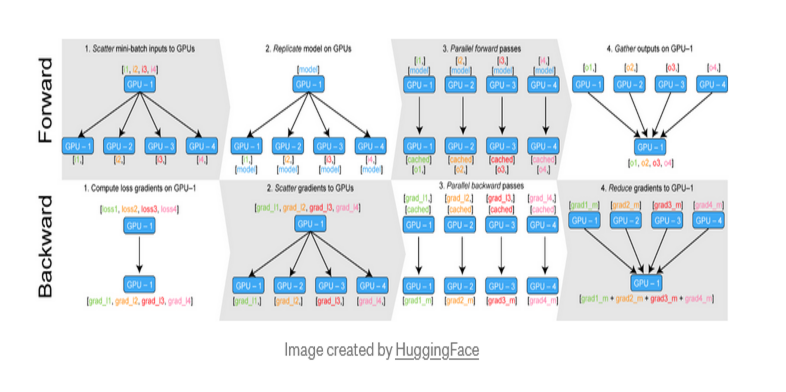
- The mini-batch is divided on GPU:0.
- Split and distribute min-batch to all available GPUs.
- Copy the model to the GPUs.
- Forward pass takes place on all GPUs.
- Compute loss in relation to network outputs on GPU:0, as well as return losses to the various GPUs. Gradients should be calculated on each GPU.
- Summation of gradients on GPU:0 and apply the optimizer to update the model.
It is worth noting that the concerns discussed here solely apply to autocast. GradScaler's behavior remains unchanged. It doesn't matter whether torch.nn.DataParallel creates threads for each device to conduct the forward pass. The autocast state is communicated in each one, and the following will work:
model = Model_m()
p_model = nn.DataParallel(model)

# Sets autocast in the main thread
with autocast():
    # There will be autocasting in p_model.
    output = p_model(input)
    # loss_fn also autocast
    loss = loss_fn(output)
DistributedDataParallel, one GPU per process
The documentation for torch.nn.parallel.DistributedDataParallel advises using one GPU per process for best performance. In this situation, DistributedDataParallel does not launch threads internally; hence the use of autocast and GradScaler is not affected.
DistributedDataParallel, multiple GPUs per process
Here torch.nn.parallel.DistributedDataParallel may spawn a side thread to run the forward pass on each device, like torch.nn.DataParallel. The fix is the same: apply autocast as part of your model’s forward method to ensure it’s enabled in side threads.
Conclusion
In this article, we have :
- Introduced Apex.
- Seen how Amps Work.
- Seen how to perform gradient scaling, gradient clipping, gradient accumulation and gradinet penalty.
- Seen how we can work with multiple models, losses and optimizers.
- Seen how we can perform DataParallel in a single process when working with mutiple GPU.
Be sure to check out the Gradient Notebook version of this code using the link at the top of the page, and see a worked example from Torch's Michael Carrili.
References
https://developer.nvidia.com/blog/apex-pytorch-easy-mixed-precision-training/
https://pytorch.org/docs/stable/notes/amp_examples.html
https://analyticsindiamag.com/pytorch-mixed-precision-training/
https://nvidia.github.io/apex/amp.html
https://kozodoi.me/python/deep learning/pytorch/tutorial/2021/02/19/gradient-accumulation.html
https://towardsdatascience.com/how-to-scale-training-on-multiple-gpus-dae1041f49d2