
Bring this project to life
Pooling operations have been a mainstay in convolutional neural networks for some time. While processes like max pooling and average pooling have often taken more of the center stage, their less known cousins global max pooling and global average pooling have become equally as important. In this article, we will be exploring what the global variants of the two common pooling techniques entail and how they compare to one another.
#  article dependencies
import torch
import torch.nn as nn
import torch.nn.functional as F
import torchvision
import torchvision.transforms as transforms
import torchvision.datasets as Datasets
from torch.utils.data import Dataset, DataLoader
import numpy as np
import matplotlib.pyplot as plt
import cv2
from tqdm.notebook import tqdm
import seaborn as sns
from torchvision.utils import make_grid
if torch.cuda.is_available():
device = torch.device('cuda:0')
print('Running on the GPU')
else:
device = torch.device('cpu')
print('Running on the CPU')The Classical Convolutional Neural Network
Many beginners in computer vision often get introduced to convolutional neural networks as the ideal neural network for image data as it retains the spatial structure of the input image while learning/extracting features from them. By doing so it is able to learn relationships between neighboring pixels and the position of objects in the image thereby making it a very powerful neural network.
A multi layer perceptron would also work in an image classification context, but its performance will be severely degraded compared to its convnet counterpart simply because it immediately destroys the spatial structure of the image by flattening/vectorizing it, thereby removing most of the relationship between neighboring pixels.
Feature Extractor & Classifier Combo
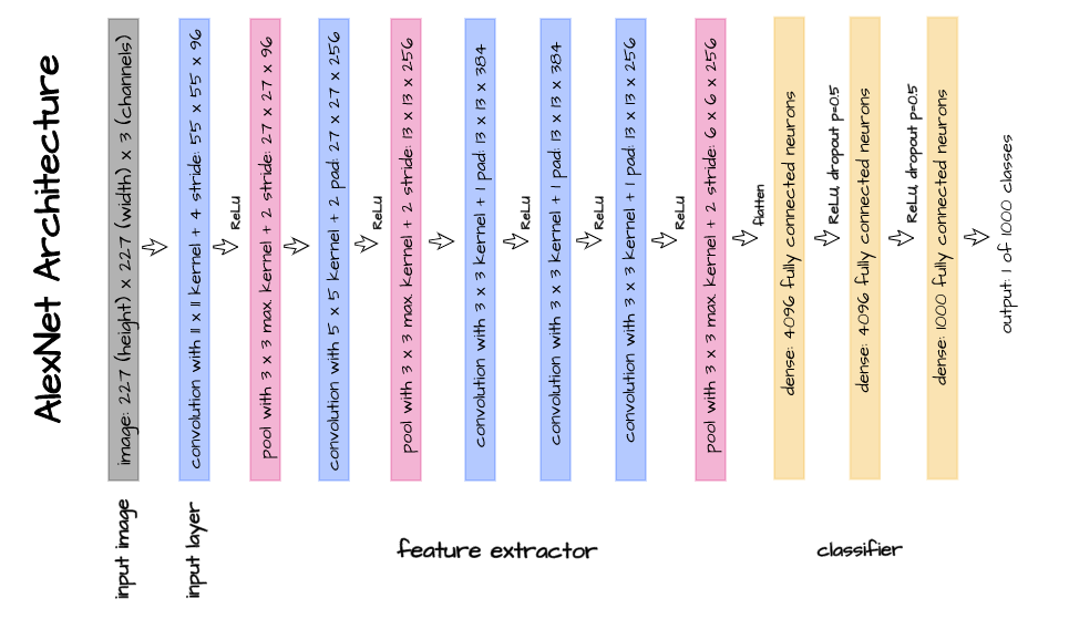
Many classical convolutional neural networks are actually a combination of convnets and MLPs. Looking at the architectures of LeNet and AlexNet for instance, one can distinctively see that their architectures are just a couple of convolution layers with linear layers attached at the end.
This configuration makes a lot of sense, it allowed the convolution layers to do what they do best which is extracting features in data with two spatial dimensions. Afterwards the extracted features are passed onto linear layers so they also can do what they are great at, finding relationships between feature vectors and targets.
A Flaw in the Design
The problem with this design is that linear layers have a very high propensity to overfit to data. Dropout regularization was introduced to help mitigate this problem but a problem it remained nonetheless. Furthermore, for a neural network which prides itself on not destroying spatial structures, the classical convnet still did it anyway, albeit deeper into the network and to a lesser degree.
Modern Solutions to a Classical Problem
In order to prevent this overfitting issue in convnets, the logical next step after trying dropout regularization was to completely get rid of the linear layers all together. If the linear layers are to be excluded, an entirely new way of down-sampling feature maps and producing a vector representation of equal size to the number of classes in question is to be sought. This exactly is where global pooling comes in.
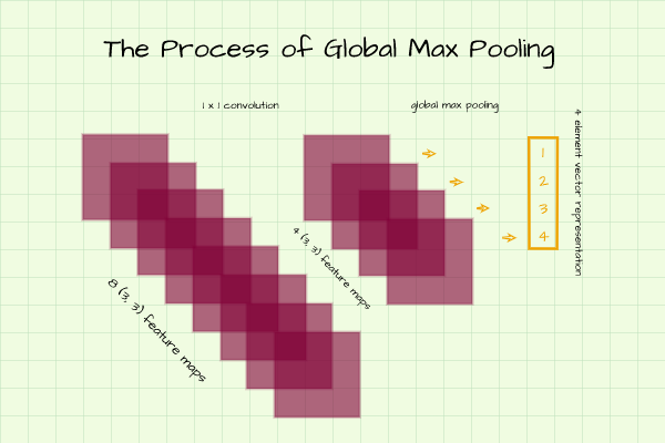
Consider a 4 class classification task, while 1 x 1 convolution layers will help to down-sample feature maps until they are 4 in number, global pooling will help to create a 4 element long vector representation which can then be used by the loss function in calculating gradients.
Global Average Pooling
Still on the same classification task described above, imagine a scenario where we feel our convolution layers are at an adequate depth but we have 8 feature maps of size (3, 3). We can utilize a 1 x 1 convolution layer in order to down-sample the 8 feature maps to 4. Now we have 4 matrices of size (3, 3) when what we actually need is a vector of 4 elements.
One way to derive a 4 element vector from these feature maps is to compute the average of all pixels in each feature map and return that as a single element. This is essentially what global average pooling entails.

Global Max Pooling
Just like the scenario above where we would like to produce a 4 element vector from 4 matrices, in this case instead of taking the average value of all pixels in each feature map, we take the maximum value and return that as an individual element in the vector representation of interest.
Benchmarking Global Pooling Methods
The benchmarking objective here is to compare both global pooling techniques based on their performance when used to generate classification vector representations. The dataset to be used for benchmarking is the FashionMNIST dataset which contains 28 pixel by 28 pixel images of common fashion items.
#  loading training data
training_set = Datasets.FashionMNIST(root='./', download=True,
                                      transform=transforms.ToTensor())

#  loading validation data
validation_set = Datasets.FashionMNIST(root='./', download=True, train=False,
transform=transforms.ToTensor())| Label | Description |
|---|---|
| 0 | T-Shirt |
| 1 | Trouser |
| 2 | Pullover |
| 3 | Dress |
| 4 | Coat |
| 5 | Sandal |
| 6 | Shirt |
| 7 | Sneaker |
| 8 | Bag |
| 9 | Ankle boot |
Convnet with Global Average Pooling
The convnet defined below makes use of a 1 x 1 convolution layer in tandem with global average pooling instead of linear layers in producing a 10 element vector representation without regularization. Concerning the implementation of global average pooling in PyTorch, all that needs to be done is to utilize the regular average pooling class but use a kernel/filter equal in size to the size of each individual feature map. To illustrate, the feature maps coming out of layer 6 are of size (3, 3) so in order to perform global average pooling, a kernel of size 3 is used. Note: simply taking the average value of each feature map will yield the same result.
class ConvNet_1(nn.Module):
  def __init__(self):
    super().__init__()
    self.network = nn.Sequential(
        #  layer 1
        nn.Conv2d(1, 8, 3, padding=1),
        nn.ReLU(), #  feature map size = (28, 28)
        #  layer 2
        nn.Conv2d(8, 8, 3, padding=1),
        nn.ReLU(),
        nn.MaxPool2d(2), #  feature map size = (14, 14)
        #  layer 3
        nn.Conv2d(8, 16, 3, padding=1),
        nn.ReLU(), #  feature map size = (14, 14)
        #  layer 4
        nn.Conv2d(16, 16, 3, padding=1),
        nn.ReLU(),
        nn.MaxPool2d(2), #  feature map size = (7, 7)
        #  layer 5
        nn.Conv2d(16, 32, 3, padding=1),
        nn.ReLU(), #  feature map size = (7, 7)
        #  layer 6
        nn.Conv2d(32, 32, 3, padding=1),
        nn.ReLU(),
        nn.MaxPool2d(2), #  feature map size = (3, 3)
        #  output layer
        nn.Conv2d(32, 10, 1),
        nn.AvgPool2d(3)
    )

  def forward(self, x):
    x = x.view(-1, 1, 28, 28)
    output = self.network(x)
    output = output.view(-1, 10)
    return torch.sigmoid(output)
Convnet with Global Max Pooling
ConvNet_2 below on the other hand replaces linear layers with a 1 x 1 convolution layer working in tandem with global max pooling in order to produce a 10 element vector without regularization. Similar to global average pooling, to implement global max pooling in PyTorch, one needs to use the regular max pooling class with a kernel size equal to the size of the feature map at that point. Note: simply deriving the maximum pixel value in each feature map would yield the same results.
class ConvNet_2(nn.Module):
  def __init__(self):
    super().__init__()
    self.network = nn.Sequential(
        #  layer 1
        nn.Conv2d(1, 8, 3, padding=1),
        nn.ReLU(), #  feature map size = (28, 28)
        #  layer 2
        nn.Conv2d(8, 8, 3, padding=1),
        nn.ReLU(),
        nn.MaxPool2d(2), #  feature map size = (14, 14)
        #  layer 3
        nn.Conv2d(8, 16, 3, padding=1),
        nn.ReLU(), #  feature map size = (14, 14)
        #  layer 4
        nn.Conv2d(16, 16, 3, padding=1),
        nn.ReLU(),
        nn.MaxPool2d(2), #  feature map size = (7, 7)
        #  layer 5
        nn.Conv2d(16, 32, 3, padding=1),
        nn.ReLU(), #  feature map size = (7, 7)
        #  layer 6
        nn.Conv2d(32, 32, 3, padding=1),
        nn.ReLU(),
        nn.MaxPool2d(2), #  feature map size = (3, 3)
        #  output layer
        nn.Conv2d(32, 10, 1),
        nn.MaxPool2d(3)
    )

  def forward(self, x):
    x = x.view(-1, 1, 28, 28)
    output = self.network(x)
    output = output.view(-1, 10)
    return torch.sigmoid(output)
Convolutional Neural Network Class
The below defined class contains the training and classification functions to be used for the training and utilizing convnets.
class ConvolutionalNeuralNet():
  def __init__(self, network):
    self.network = network.to(device)
    self.optimizer = torch.optim.Adam(self.network.parameters(), lr=3e-4)

  def train(self, loss_function, epochs, batch_size,
            training_set, validation_set):

    #  creating log
    log_dict = {
        'training_loss_per_batch': [],
        'validation_loss_per_batch': [],
        'training_accuracy_per_epoch': [],
        'validation_accuracy_per_epoch': []
    }

    #  defining weight initialization function
    def init_weights(module):
      if isinstance(module, nn.Conv2d):
        torch.nn.init.xavier_uniform_(module.weight)
        module.bias.data.fill_(0.01)

    #  defining accuracy function
    def accuracy(network, dataloader):
      total_correct = 0
      total_instances = 0
      for images, labels in tqdm(dataloader):
        images, labels = images.to(device), labels.to(device)
        predictions = torch.argmax(network(images), dim=1)
        correct_predictions = sum(predictions==labels).item()
        total_correct+=correct_predictions
        total_instances+=len(images)
      return round(total_correct/total_instances, 3)

    #  initializing network weights
    self.network.apply(init_weights)

    #  creating dataloaders
    train_loader = DataLoader(training_set, batch_size)
    val_loader = DataLoader(validation_set, batch_size)

    for epoch in range(epochs):
      print(f'Epoch {epoch+1}/{epochs}')
      train_losses = []

      #  training
      print('training...')
      for images, labels in tqdm(train_loader):
        #  sending data to device
        images, labels = images.to(device), labels.to(device)
        #  resetting gradients
        self.optimizer.zero_grad()
        #  making predictions
        predictions = self.network(images)
        #  computing loss
        loss = loss_function(predictions, labels)
        log_dict['training_loss_per_batch'].append(loss.item())
        train_losses.append(loss.item())
        #  computing gradients
        loss.backward()
        #  updating weights
        self.optimizer.step()
      with torch.no_grad():
        print('deriving training accuracy...')
        #  computing training accuracy
        train_accuracy = accuracy(self.network, train_loader)
        log_dict['training_accuracy_per_epoch'].append(train_accuracy)

      #  validation
      print('validating...')
      val_losses = []

      with torch.no_grad():
        for images, labels in tqdm(val_loader):
          #  sending data to device
          images, labels = images.to(device), labels.to(device)
          #  making predictions
          predictions = self.network(images)
          #  computing loss
          val_loss = loss_function(predictions, labels)
          log_dict['validation_loss_per_batch'].append(val_loss.item())
          val_losses.append(val_loss.item())
        #  computing accuracy
        print('deriving validation accuracy...')
        val_accuracy = accuracy(self.network, val_loader)
        log_dict['validation_accuracy_per_epoch'].append(val_accuracy)

      train_losses = np.array(train_losses).mean()
      val_losses = np.array(val_losses).mean()

      print(f'training_loss: {round(train_losses, 4)}  training_accuracy: '+
      f'{train_accuracy}  validation_loss: {round(val_losses, 4)} '+
      f'validation_accuracy: {val_accuracy}\n')

    return log_dict

  def predict(self, x):
    return self.network(x)
Benchmark Results
Bring this project to life
ConvNet_1 (Global Average Pooling)
ConvNet_1 uses global average pooling in producing a classification vector. Setting parameters of interest and training for 60 epochs produces a metric log as analyzed below.
model_1 = ConvolutionalNeuralNet(ConvNet_1())

log_dict_1 = model_1.train(nn.CrossEntropyLoss(), epochs=60, batch_size=64,
                       training_set=training_set, validation_set=validation_set)
From the log obtained, both training and validation accuracy increased over the course of model training. Validation accuracy starts off at about 66% before increasing steadily to a value just under 80% by the 28th epoch. A sharp increase to a value under 85% is then observed by the 31st epoch before eventually culminating at approximately 87% by the 60th epoch.
sns.lineplot(y=log_dict_1['training_accuracy_per_epoch'], x=range(len(log_dict_1['training_accuracy_per_epoch'])), label='training')

sns.lineplot(y=log_dict_1['validation_accuracy_per_epoch'], x=range(len(log_dict_1['validation_accuracy_per_epoch'])), label='validation')

plt.xlabel('epoch')
plt.ylabel('accuracy')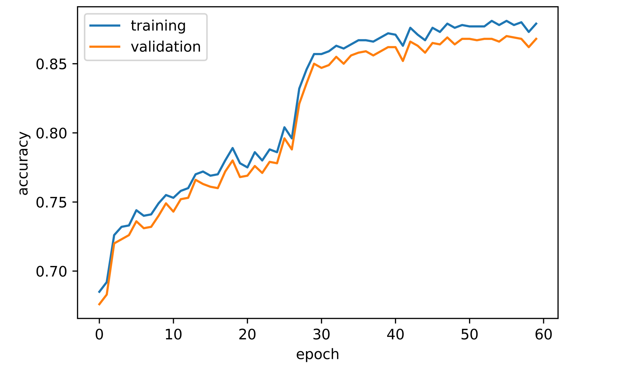
ConvNet_2 (Global Max Pooling)
ConvNet_2 utilizes global max pooling instead of global average pooling in producing a 10 element classification vector. Keeping all parameters the same and training for 60 epochs yields the metric log below.
model_2 = ConvolutionalNeuralNet(ConvNet_2())

log_dict_2 = model_2.train(nn.CrossEntropyLoss(), epochs=60, batch_size=64,
                       training_set=training_set, validation_set=validation_set)
Overall, both training and validation accuracy increased over the course of 60 epochs. Validation accuracy starts off at just under 70% before fluctuating whilst increasing steadily to a value just under 85% by the 60th epoch.
sns.lineplot(y=log_dict_2['training_accuracy_per_epoch'], x=range(len(log_dict_2['training_accuracy_per_epoch'])), label='training')

sns.lineplot(y=log_dict_2['validation_accuracy_per_epoch'], x=range(len(log_dict_2['validation_accuracy_per_epoch'])), label='validation')

plt.xlabel('epoch')
plt.ylabel('accuracy')
plt.savefig('maxpool_benchmark.png', dpi=1000)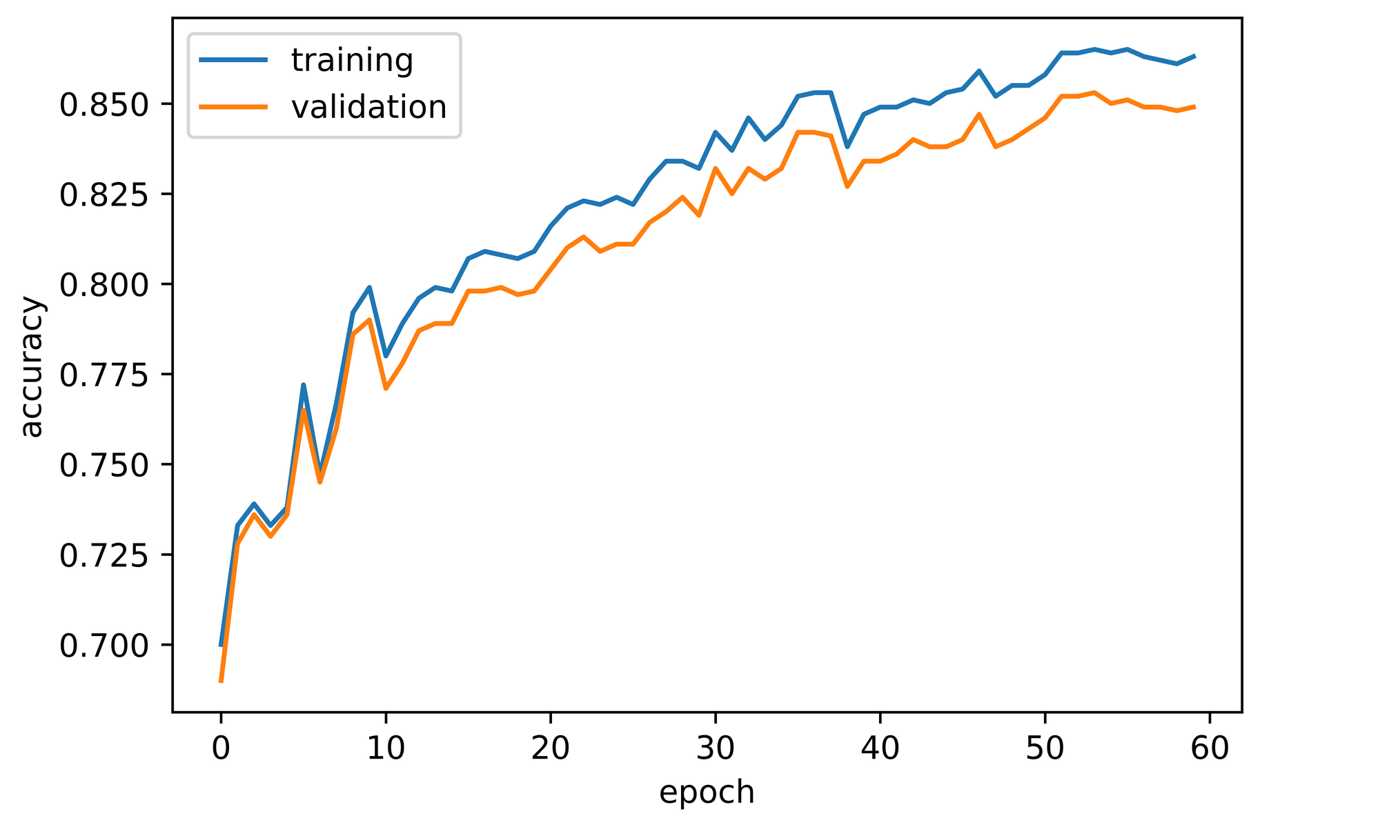
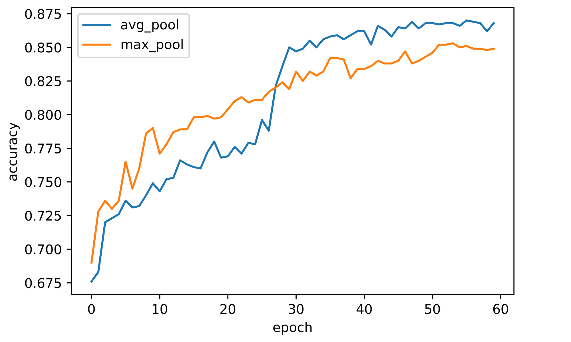
Comparing Performance
Comparing the performance of both global pooling techniques, one can easily infer that global average pooling performs better, at least on the dataset we chose to use (FashionMNIST). It seems to be quite logical really since global average pooling produces a single value which is representative of the general nature of all pixels in each feature map as opposed to global max pooling which produces a single value in isolation without regards to other pixels present in the feature map. However, to reach a more conclusive verdict, benchmarking should be done across several datasets.
Global Pooling Under the Hood
In order to develop an intuition for why global pooling actually works, we need to write a function which will enable us to visualize the output of an intermediate layer in a convolutional neural network. Many times neural networks are thought to be black box models, but there are certain ways to at least try to pry open the black box in a bid to understand what goes on inside. The function below does just that.
def visualize_layer(model, dataset, image_idx: int, layer_idx: int):
  """
  This function visulizes intermediate layers in a convolutional neural
  network defined using the PyTorch sequential class
  """
  #  creating a dataloader
  dataloader = DataLoader(dataset, 250)

  #  deriving a single batch from dataloader
  for images, labels in dataloader:
    images, labels = images.to(device), labels.to(device)
    break

  #  deriving output from layer of interest
  output = model.network.network[:layer_idx].forward(images[image_idx])
  #  deriving output shape
  out_shape = output.shape

  #  classifying image
  predicted_class = model.predict(images[image_idx])

  print(f'actual class: {labels[image_idx]}\npredicted class: {torch.argmax(predicted_class)}')

  #  visualising layer
  plt.figure(dpi=150)
  plt.title(f'visualising output')
  plt.imshow(np.transpose(make_grid(output.cpu().view(out_shape[0], 1,
                                                        out_shape[1],
                                                        out_shape[2]),
                                    padding=2, normalize=True), (1,2,0)))
  plt.axis('off')
In order to use the function, the parameters should be properly understood. The model refers to a convolution neural network instantiated the same way we have done in this article, other types will not work with this function. Dataset in this case could be any dataset, but preferably the validation set. Image_idx is the index of an image in the first batch of the dataset provided, the function defines a batch as 250 images so image_idx could range from 0 - 249. Layer_idx on the other hand does not exactly refer to convolution layers, it refers to layers as defined by the PyTorch sequential class as seen below.
model_1.network

#  output
>>>> ConvNet_1(
  (network): Sequential(
    (0): Conv2d(1, 8, kernel_size=(3, 3), stride=(1, 1), padding=(1, 1))
    (1): ReLU()
    (2): Conv2d(8, 8, kernel_size=(3, 3), stride=(1, 1), padding=(1, 1))
    (3): ReLU()
    (4): MaxPool2d(kernel_size=2, stride=2, padding=0, dilation=1, ceil_mode=False)
    (5): Conv2d(8, 16, kernel_size=(3, 3), stride=(1, 1), padding=(1, 1))
    (6): ReLU()
    (7): Conv2d(16, 16, kernel_size=(3, 3), stride=(1, 1), padding=(1, 1))
    (8): ReLU()
    (9): MaxPool2d(kernel_size=2, stride=2, padding=0, dilation=1, ceil_mode=False)
    (10): Conv2d(16, 32, kernel_size=(3, 3), stride=(1, 1), padding=(1, 1))
    (11): ReLU()
    (12): Conv2d(32, 32, kernel_size=(3, 3), stride=(1, 1), padding=(1, 1))
    (13): ReLU()
    (14): MaxPool2d(kernel_size=2, stride=2, padding=0, dilation=1, ceil_mode=False)
    (15): Conv2d(32, 10, kernel_size=(1, 1), stride=(1, 1))
    (16): AvgPool2d(kernel_size=3, stride=3, padding=0)
  )
)
Why Global Average Pooling Works
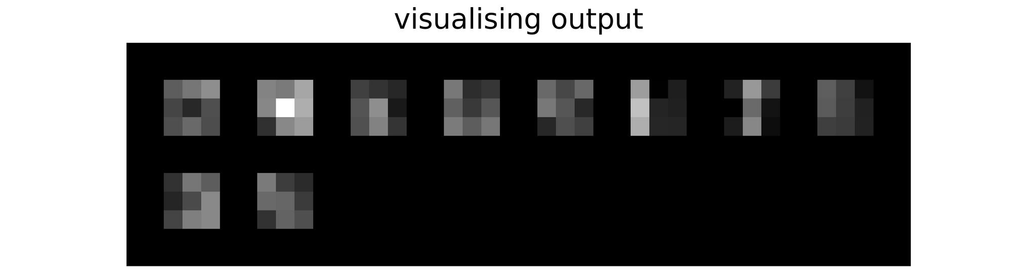
In order to understand why global average pooling works, we need to visualize the output of the output layer right before global average pooling is done, this corresponds to layer 15 so we need to grab/index layers up till layer 15 which implies that layer_idx=16. Using model_1 (ConvNet_1), we produce the results below.
visualize_layer(model=model_1, dataset=validation_set, image_idx=2, layer_idx=16)

#  output
>>>> actual class: 1
>>>> predicted class: 1
When we visualize the output of image 3 (index 2) just before global average pooling, we can see that the model has predicted it's class correctly as class 1 (trouser) as seen above. Looking at the visualization, we can see that the feature map at index 1 has the brightest pixels on average when compared to the other feature maps. In other words, the convnet has learnt to classify images by 'switching on' more pixels in the feature map of interest just before global average pooling. When global average pooling is then done, the highest valued element will be located at index 1 hence why it is chosen as the correct class.
Why Global Max Pooling Works
Keeping all parameters the same but using model_2 (ConvNet_2) in this instance, we obtain the results below. Again, the convnet correctly classifies this image as belonging to class 1. Looking at the visualization produced, we can see that the feature map at index 1 contains the brightest pixel.
The convnet has in this case learnt to classify images by 'switching on' pixels the brightest in the feature map of interest just before global max pooling.
visualize_layer(model=model_2, dataset=validation_set, image_idx=2, layer_idx=16)

#  output
>>>> actual class: 1
>>>> predicted class: 1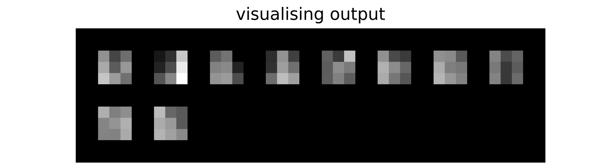
Final Remarks
In this article, we explored what global average and max pooling entail. We discussed why they have come to be used and how they measure up against one another. We also developed an intuition into why they work by performing a biopsy of our convnets and visualizing intermediate layers.