Play Super Mario Bros with a Double Deep Q-Network

As cool as neural networks are, the first time that I felt like I was building true AI was not when working on image classification or regression problems, but when I started working on deep reinforcement learning. In this article I would like to share that experience with you. By the end of the tutorial, you will have a working PyTorch reinforcement learning agent that can make it through the first level of Super Mario Bros (NES).

This tutorial is broken into 3 parts:

1. Introduction to reinforcement learning
2. The Super Mario Bros (NES) environment
3. Building an agent that can get through this environment

You can run the code for free on the ML Showcase.

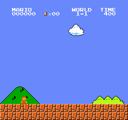
By the end of this tutorial, you will have built an agent that can do this:

Pre-requisites

• Have a working knowledge of deep learning and convolutional neural networks
• Have Python 3+ and a Jupyter Notebook
• Optional: be comfortable with PyTorch

What is reinforcement learning?

Reinforcement learning is the family of learning algorithms in which an agent learns from its environment by interacting with it. What does it learn? Informally, an agent learns to take actions that bring it from its current state to the best (optimal) reachable state.

I find that examples always help. Examine the following 3×3 grid:

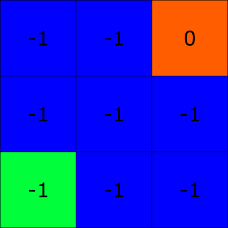
This grid is our agent's environment. Each square in this environment is called a state, and an environment will always have a start and end state which you can see highlighted in green and red, respectively. Much like a human, our agent will learn from repetition in a process called an episode. At the start of an episode an agent will begin at the start state, and it will keep making actions until it arrives at the end state. Once the agent makes it to the end state the episode will terminate, and a new one will begin with the agent once again beginning from the start state.

Here I've just given you a grid, but you can imagine more realistic examples. Imagine you're in a grocery store and you look at your shopping list: you need to buy dried rosemary. Your start state would be your location when you enter the store. The first time you try to find rosemary you might be a bit lost, and you probably won't move the most direct way through the store to find the "Herbs and Spices" aisle. But on each subsequent visit you'll get better and better at finding it, until you reach the point where you can move directly to the correct aisle when you walk in.

When an agent lands on a state it accumulates the reward associated with that state, and a good agent wants to maximize the accumulated discounted reward along an episode (I'll explain what discounted means later). Suppose our agent can move vertically, horizontally, and diagonally. Based on this information, you can see that the best way for the agent to make it to the end state is to move diagonally (directly towards it), since it would accumulate a reward of -1 + 0 = -1. If the agent would move in any other way towards the end state, it would accumulate a reward less than -1. For example, if the agent were to move right, right, up, and then up once more, it would get a reward of -1 + (-1) + (-1) + 0 = -3, which is less than -1.  Moving diagonally is therefore called the optimal policy π_*, where π is a function which takes in a state and outputs the action the agent will take from that given state. You can logically deduce the best policy for this simple grid, but how would we solve this problem using reinforcement learning? Since this article is about deep q-learning, we first need to understand state-action values.

Q-learning

We mentioned that for every state in the above grid problem, the agent can move to any state that is touching the current state; so our set of actions for every state is vertical, horizontal, and diagonal. A state-action value is the quality of being on a particular state and taking a particular action off of that state. Every single state and action pair, except for the end state, should have a value. We denote these state-action values as Q(s, a) (the quality of the state-action pair), and all state-action values together form something called a Q-table. Once the Q-table is learned, if an agent is on a particular state s, it will take the action a from s such that Q(s, a) has the highest value. Mathematically, if an agent is on state s, it will take argmax_aQ(s, a). But how are these values learned? Q-learning uses a variation of the Bellman-update equation, and is more specifically a type of temporal difference learning.

The Q-learning update equation is:

Q(s_t, a_t)←Q(s_t, a_t) + α(r_t+1 + γmax_aQ(s_t+1, a) - Q(s_t, a_t))

Essentially, this equation says that the quality of being on state s_t and taking action a_t is not just defined by the immediate reward that you get from taking that action, but also by the best possible move you can take on the state s_t+1 after landing on it (the max_aQ(s_t+1, a) term). The γ parameter is called the discount factor, and is a value between 0 and 1 which defines how important future states should be. The value α is called the learning rate, and tells us how large to make our Q-updates. This should make you recall when I mentioned that the goal of a reinforcement learning agent is to maximize the accumulated discounted reward.

If we re-rewrite this equation as:

Q(s_t, a_t)←Q(s_t, a_t) + αδ

You will notice that when δ≈0 the algorithm converges, since we are no longer updating Q(s_t, a_t). This value, δ, is known as the temporal difference error, and the job of Q-learning is to make that value go to 0.

Now, let's use Q-learning to solve the grid problem in Python. The main function to solve the grid problem is:

def train_agent():
    num_episodes = 2000
    agent = Agent()
    env = Grid()
    rewards = []
    for _ in range(num_episodes):
        state = env.reset()
        episode_reward = 0
        while True:
            action_id, action = agent.act(state)
            next_state, reward, terminal = env.step(action)
            episode_reward += reward
            
            agent.q_update(state, action_id, reward, next_state, terminal)
            state = next_state
            
            if terminal:
                break
        rewards.append(episode_reward)
    
    plt.plot(rewards)
    plt.show()
    return agent.best_policy()
    
print(train_agent())

The idea is really simple. Given a state, the agent takes the action that has the highest value, and after taking that action, the Q-table gets updated using the Bellman equation above. The next state then becomes the current state, and the agent continues using this pattern. If the agent lands on the terminal state then a new episode starts. The Q-table update method is simply:

class Agent():
    ...
    def q_update(self, state, action_id, reward, next_state, terminal):
        ...
        if terminal:
            target = reward
        else:
            target = reward + self.gamma*max(self.q_table[next_state])
        
        td_error = target - self.q_table[state, action_id]
        self.q_table[state, action_id] = self.q_table[state, action_id] + self.alpha*td_error
    ...

After running for 1000 episodes, I got the final policy to be:

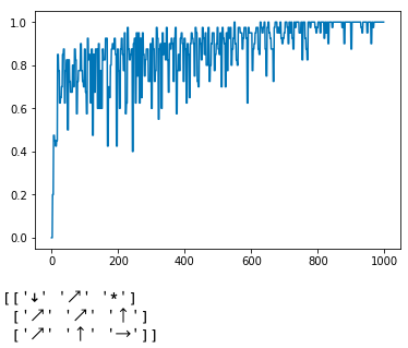
You may notice that some of the arrows don't make sense. For example, if you were at the top left of the grid, shouldn't the agent want to move right instead of down? Just remember, Q-learning is a greedy algorithm; the agent does not make it to the top left enough times to figure out what the best policy is from that position. What matters is that from the start state, it figured out the best policy is to move diagonally.

Double Q-Learning

There is one major issue with Q-learning that we need to deal with: over-estimation bias, which means that the Q-values learned are actually higher than they should be. Mathematically, max_aQ(s_t+1, a) converges to E(max_aQ(s_t+1, a)), which is higher than max_a(E(Q(s_t+1, a)), the true Q-value (I won't prove that here). To get more accurate Q-values, we use something called double Q-learning. In double Q-learning we have two Q-tables: one which we use for taking actions, and another specifically for use in the Q-update equation. The double Q-learning update equation is:

Q*(s_t, a_t)←Q*(s_t, a_t) + α(r_t+1 + γmax_aQ^T(s_t+1, a) - Q*(s_t, a_t))

where Q^* is the Q table that gets updated, and Q^T is the target table. Q^T copies the values of Q^* every n steps.

Below are a few code snippets to demonstrate the changes:

class AgentDoubleQ():
    ...
    def q_update(self, state, action_id, reward, next_state, terminal):
        state = state[0]*3 + state[1]
        next_state = next_state[0]*3 + next_state[1]
        if terminal:
            target = reward
        else:
            target = reward + self.gamma*max(self.q_target[next_state])
        
        td_error = target - self.q_table[state, action_id]
        self.q_table[state, action_id] = self.q_table[state, action_id] + self.alpha*td_error
    
    def copy(self):
        self.q_target = copy.deepcopy(self.q_table)
    ...

def train_agent_doubleq():
    ...
    while True:
        action_id, action = agent.act(state)
        next_state, reward, terminal = env.step(action)
            
        num_steps += 1
        if num_steps % agent.copy_steps == 0:
            agent.copy()
            
        episode_reward += reward
            
        agent.q_update(state, action_id, reward, next_state, terminal)
        state = next_state
            
        if terminal:
            break
    ...

Below is a plot of normalized rolling average reward over 1000 episodes.

From this plot, it might be hard to tell what the advantage of double Q-learning is over Q-learning, but that's because our state space is really small (only 9 states). When we get much larger state spaces, double Q-learning really helps to speed up convergence.

Super Mario Bros (NES)

Now that you have a brief overview of reinforcement learning, let's build our agent that can make it through the first level of Super Mario Bros (NES). We will be using the gym-super-mario-bros library, built on top of the OpenAI gym. For those not familiar with gym, it is an extremely popular Python library that provides ML enthusiasts with a set of environments for reinforcement learning. Below is the code snippet to instantiate our environment and view the size of each state, as well as the action space:

import gym_super_mario_bros

env = gym_super_mario_bros.make('SuperMarioBros-1-1-v0')
print(env.observation_space.shape)  # Dimensions of a frame
print(env.action_space.n)  # Number of actions our agent can take

You will see that the observation space shape is 240 × 256 × 3 (240 and 256 represent the height and width respectively, and 3 represents the 3 color channels). The agent can take 256 different possible actions. In double deep Q-learning, reducing the state and action space sizes speeds up convergence of our model. A nice part of gym is that we can use gym's Wrapper class to change the default settings originally given to us. Below I have defined a few classes that will help our agent learn faster.

def make_env(env):
    env = MaxAndSkipEnv(env)
    env = ProcessFrame84(env)
    env = ImageToPyTorch(env)
    env = BufferWrapper(env, 4)
    env = ScaledFloatFrame(env)
    return JoypadSpace(env, RIGHT_ONLY)

This function applies 6 different transformations to our environment:

1. Every action the agent makes is repeated over 4 frames
2. The size of each frame is reduced to 84×84
3. The frames are converted to PyTorch tensors
4. Only every fourth frame is collected by the buffer
5. The frames are normalized so that pixel values are between 0 and 1
6. The number of actions is reduced to 5 (such that the agent can only move right)

Building an agent for Super Mario Bros (NES)

Let's finally get to what makes deep Q-learning "deep". From the way we've set up our environment, a state is a list of 4 contiguous 84×84 pixel frames, and we have 5 possible actions. If we were to make a Q-table for this environment, the table would have 5×256^84×84×4 values, since there are 5 possible actions for each state, each pixel has intensities between 0 and 255, and there are 84×84×4 pixels in a state. Clearly, storing a Q-table that large is impossible, so we have to resort to function approximation in which we use a neural network to approximate the Q-table; that is, we will use a neural network to map a state to its state-action values.

In tabular (table-based) double Q-learning, recall that the update equation is:

Q^*(s_t, a_t)←Q^*(s_t, a_t) + α(r_t+1 + γmax_aQ_θ(s_t+1, a) - Q^*(s_t, a_t)).

r_t+1 + γmax_aQ_θ(s_t+1, a) is considered our target, and Q^*(s_t, a_t) is the value predicted by our network. Using some type of distance-based loss function (mean-squared error, Huber loss, etc.), we can optimize the weights of our deep Q-networks using gradient descent.

Before getting to the details of how we train our agent, let's first build the DQN architecture that we will use as a function approximator.

class DQNSolver(nn.Module):

    def __init__(self, input_shape, n_actions):
        super(DQNSolver, self).__init__()
        self.conv = nn.Sequential(
            nn.Conv2d(input_shape[0], 32, kernel_size=8, stride=4),
            nn.ReLU(),
            nn.Conv2d(32, 64, kernel_size=4, stride=2),
            nn.ReLU(),
            nn.Conv2d(64, 64, kernel_size=3, stride=1),
            nn.ReLU()
        )

        conv_out_size = self._get_conv_out(input_shape)
        self.fc = nn.Sequential(
            nn.Linear(conv_out_size, 512),
            nn.ReLU(),
            nn.Linear(512, n_actions)
        )

    def _get_conv_out(self, shape):
        o = self.conv(torch.zeros(1, *shape))
        return int(np.prod(o.size()))

    def forward(self, x):
        conv_out = self.conv(x).view(x.size()[0], -1)
        return self.fc(conv_out)

Our DQN is a convolutional neural net with 3 convolutional layers and two linear layers. It takes two arguments: input_shape and n_actions. Of course, the input shape we will provide is 4×84×84, and there are 5 actions. We have chosen to use a convolutional neural net because they are ideal for image-based regression.

Now that we have our neural net architecture set up, let's go through the "main function" of our code.

def run():
    env = gym_super_mario_bros.make('SuperMarioBros-1-1-v0')
    env = make_env(env)  # Wraps the environment so that frames are grayscale 
    observation_space = env.observation_space.shape
    action_space = env.action_space.n
    agent = DQNAgent(state_space=observation_space,
                     action_space=action_space,
                     max_memory_size=30000,
                     batch_size=32,
                     gamma=0.90,
                     lr=0.00025,
                     exploration_max=0.02,
                     exploration_min=0.02,
                     exploration_decay=0.99)
    
    num_episodes = 10000
    env.reset()
    total_rewards = []
    
    for ep_num in tqdm(range(num_episodes)):
        state = env.reset()
        state = torch.Tensor([state])
        total_reward = 0
        while True:
            action = agent.act(state)
            
            state_next, reward, terminal, info = env.step(int(action[0]))
            total_reward += reward
            state_next = torch.Tensor([state_next])
            reward = torch.tensor([reward]).unsqueeze(0)
            
            terminal = torch.tensor([int(terminal)]).unsqueeze(0)
            agent.remember(state, action, reward, state_next, terminal)
            agent.experience_replay()
            
            state = state_next
            if terminal:
                break
        
        total_rewards.append(total_reward)

        print("Total reward after episode {} is {}".format(ep_num + 1, total_rewards[-1]))
        num_episodes += 1    

It looks almost identical to the main function of the grid problem, right? The only differences you might see are the remember and experience_replay methods. In typical supervised learning, a neural network uses batches of data to update its weights. In deep Q-learning the idea is the same, except these batches of data are called batches of experiences, where an experience is a (state, action, reward, next_state, terminal) tuple. Instead of throwing away experiences like we did in the grid problem, we can store them in a buffer to use later with the remember method. In the experience_replay method, the agent just has to sample a batch of experiences and use the double Q-update equation to update the network weights.

Now, let's go over the most important methods of our agent: remember, recall, and experience_replay.

class DQNAgent:
    ...
    def remember(self, state, action, reward, state2, done):
        self.STATE_MEM[self.ending_position] = state.float()
        self.ACTION_MEM[self.ending_position] = action.float()
        self.REWARD_MEM[self.ending_position] = reward.float()
        self.STATE2_MEM[self.ending_position] = state2.float()
        self.DONE_MEM[self.ending_position] = done.float()
        self.ending_position = (self.ending_position + 1) % self.max_memory_size  # FIFO tensor
        self.num_in_queue = min(self.num_in_queue + 1, self.max_memory_size)
        
    def recall(self):
        # Randomly sample 'batch size' experiences
        idx = random.choices(range(self.num_in_queue), k=self.memory_sample_size)
        
        STATE = self.STATE_MEM[idx].to(self.device)
        ACTION = self.ACTION_MEM[idx].to(self.device)
        REWARD = self.REWARD_MEM[idx].to(self.device)
        STATE2 = self.STATE2_MEM[idx].to(self.device)
        DONE = self.DONE_MEM[idx].to(self.device)
        
        return STATE, ACTION, REWARD, STATE2, DONE
        
    def experience_replay(self):
        
        if self.step % self.copy == 0:
            self.copy_model()

        if self.memory_sample_size > self.num_in_queue:
            return

        STATE, ACTION, REWARD, STATE2, DONE = self.recall()
        
        self.optimizer.zero_grad()
        # Double Q-Learning target is Q*(S, A) <- r + γ max_a Q_target(S', a)
        target = REWARD + torch.mul((self.gamma * 
        self.target_net(STATE2).max(1).values.unsqueeze(1)), 
        1 - DONE)

        current = self.local_net(STATE).gather(1, ACTION.long()) # Local net approximation of Q-value
        
        loss = self.l1(current, target)
        loss.backward() # Compute gradients
        self.optimizer.step() # Backpropagate error

        ...
    ...

So what's going on here?  In the remember method, we just push an experience onto the buffer so that we can use that data for later. The buffer has a fixed size, so it has a deque data structure. The recall method just samples a batch of experiences from memory. In the experience_replay method, you will notice that we have two Q-networks: target net and local net. This is analogous to how we had the target and local Q-tables for the grid problem. We copy the local weights to be the target weights, sample from our memory buffer, and just apply the Double Q-learning update equation. This method is what will allow our agent to learn.

Running the code

You can run the full code for free on the ML Showcase.

The code has options to allow the user to run either deep Q-learning or double deep Q-learning, however for comparison, here are a few plots that compare the DQN performance to the DDQN performance:

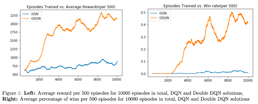
You will notice that the DQN at 10,000 episodes has the same performance as the DDQN in just 1,000 episodes (look at the average reward plot on the left). The code for the single DQN is available just for educational purposes; I highly recommend you stick to training the DDQN.

Conclusion

Congratulations! If you're anything like me, seeing Mario consistently make it through the level will give you such a rush that you'll want to jump to new deep reinforcement learning projects. There are topics that I did not cover in this post, such as value iteration, on- vs off-policy learning, Markov Decision Processes, and much, much more. However, this article was meant to get people excited about the awesome opportunities that deep reinforcement learning has to offer. Take care, and see you in my next post!