
Bring this project to life
Oftentimes when tackling image classification tasks in deep learning there aren't the same number of images for each class in the training set. This scenario is termed class imbalance, and is an extremely common problem to find when sourcing data for deep learning tasks.
In this article, we will be taking a look at how and if class imbalance affects model performance, as well as its influence on the choice of evaluation metrics.
Why Class Imbalance?
In most cases where there is a class imbalance in datasets it's often because it's unavoidable. Consider a case where one would like to curate an audio dataset for detecting mechanical faults in car engines for instance. Clearly, two audio classes will be required, one for engines in perfect working condition and another for engines in defective state.
It goes without saying that there will be more audio samples for engines in perfect working condition compared to engines in a defective state and collected data will most likely than not reflect this pattern as well. This in essence sets up a class imbalance where the condition which we are trying to model ends up as the minority class. This scenario is also apparent in datasets for spam detection, fraudulent transaction detection and lots more.
Model Objectives
When building models for a specific task there is oftentimes a clear objective/goal looking to be archived. So to simplify things a bit, let's consider a binary classification task, i.e. with only two classes. Binary classification tasks may be defined/described as true/false tasks and are often labelled 1 (true/positive) or 0 (false/negative). A popular form of this task is medical imagery classification for cancer diagnostics where models are built to classify images (CT scans) as cancerous (true/positive/1) or non-cancerous (false/negative/0).
Since we know that models are never 100% accurate, in this kind of performance critical task the objective is to build a model which has a very low rate of false negative classifications. In other words, you want a model that has a very low chance of classifying cancerous images as non-cancerous. Think about it, we would not want to send a cancer patient home based on the inaccuracy of our model, that could be life threatening.
This kind of model will invariably classify borderline images as positive for cancer which will most likely yield a lot of false positive classifications. However, with an actual physician on hand to screen all positive classification by the model, the false positive classifications will eventually be weeded out. This represents a safer and more efficient tradeoff.
Evaluation Metrics
In this section, we shall take a look at some evaluation metrics in classification tasks which will make it easier for us to assess how well a model fits the objective at hand.
Accuracy
Perhaps the most popular of classification metrics, accuracy is the proportion of correctly classified instances of data to the total number of instances classified. It is typically a pointer to how well a model generalizes to data instances which it was trained on but in most cases it doesn't tell the whole story. It is measured on a scale of 0-100 or 0-1 (normalized).

Recall
Also measured on a similar scale as accuracy, recall is the ratio of true positive classifications to the sum of true positive and false negative classifications. Recall isn't exactly concerned about how well a model fits to data; rather, it is more concerned with measuring the tendency of a model to dole out false negative classifications.

The closer a recall score is to 100 the less likely a model is to produce false negative classifications. As regards the medical imagery task described in the previous section where the goal was to minimize false negatives, a model with high recall is to be sought.
Precision
Measured on a scale of 0-100 similar to the two metrics previously touched on, precision is defined as the ratio of true positive classifications to the sum of true positive and false positive classifications. As sort of an inverse of recall, precision measures the tendency of a model to give false positive classifications. The closer a model's precision score is to 100 the less likely it is to produce false positive classifications.

F-1 Score
F-1 score is a metric which measures the balance/trade-off between precision and recall. It is an harmonic mean of the two metrics. We can use this in situations where the precision-recall tradeoff is unimportant to the model's success. Cancer diagnosis, for example, would not be the ideal place for this metric.

Setup
#  article dependencies
import torch
import torch.nn as nn
import torch.nn.functional as F
import torchvision
import torchvision.transforms as transforms
import torchvision.datasets as Datasets
from torch.utils.data import Dataset, DataLoader
import numpy as np
import matplotlib.pyplot as plt
from tqdm.notebook import tqdm
from tqdm import tqdm as tqdm_regular
import seaborn as sns
from torchvision.utils import make_grid
import random
# setting up device
if torch.cuda.is_available():
device = torch.device('cuda:0')
print('Running on the GPU')
else:
device = torch.device('cpu')
print('Running on the CPU')We need to import these packages to run this tutorial.
Evaluating the Evaluation Metrics
To make sense of these evaluation metrics, let's get hands on with a real dataset. For this purpose, we shall use the CIFAR-10 dataset loaded in the code cell below.
#  loading training data
training_set = Datasets.CIFAR10(root='./', download=True,
                              transform=transforms.ToTensor())

#  loading validation data
validation_set = Datasets.CIFAR10(root='./', download=True, train=False,
                                transform=transforms.ToTensor())
In order to set up a binary classification task, we need to extract just two of the 10 classes contained in this dataset. The code cell below contains a function which extracts images of cats and dogs. A 4:1 imbalance is then created in favor of cats in the training images (80% cats, 20% dogs). However, there is no imbalance in validation images as there are equal number of image instances.
def extract_images(dataset):
  cats = []
  dogs = []

  for idx in tqdm_regular(range(len(dataset))):
    if dataset.targets[idx]==3:
      cats.append((dataset.data[idx], 0))
    elif dataset.targets[idx]==5:
      dogs.append((dataset.data[idx], 1))
    else:
      pass
  return cats, dogs

#  extracting training images
cats, dogs = extract_images(training_set)
#  creating training data with a 80:20 imbalance in favour of cats
training_images = cats[:4800] + dogs[:1200]
random.shuffle(training_images)

#  extracting validation images
cats, dogs = extract_images(validation_set)
#  creating validation data
validation_images = cats + dogs
random.shuffle(validation_images)
Building a Detector
This section sets up an hypothetical scenario which will require us to play along a little bit. Imagine a neighborhood where the only animals present are cats and dogs. The goal here is to create a deep learning model which will work in an unmanned security system for a cat shelter. Stray cats can walk up to this security system and be allowed passage into the shelter while stray dogs are refused entry and turned back.
We can call this model a dog detector hence dogs are labelled 1 (positive) while cats are labelled 0 (negative) as seen in the code cell above. Remember that there is a 4:1 imbalance in favor of cats in our dataset. The model objective here is to create a model with a low rate of false negatives, as having a dog in a cat shelter is a bad idea. Hence, we are looking to maximize recall.
Firstly, we need to define a PyTorch dataset class so that we can create PyTorch datasets from the above defined objects.
#  defining dataset class
class CustomCatsvsDogs(Dataset):
  def __init__(self, data, transforms=None):
    self.data = data
    self.transforms = transforms

  def __len__(self):
    return len(self.data)

  def __getitem__(self, idx):
    image = self.data[idx][0]
    label = torch.tensor(self.data[idx][1])

    if self.transforms!=None:
      image = self.transforms(image)
    return(image, label)

#  creating pytorch datasets
training_data = CustomCatsvsDogs(training_images, transforms=transforms.Compose([transforms.ToTensor(),
                                                                                 transforms.Normalize((0.5, 0.5, 0.5), (0.5, 0.5, 0.5))]))
validation_data = CustomCatsvsDogs(validation_images, transforms=transforms.Compose([transforms.ToTensor(),
                                                                                     transforms.Normalize((0.5, 0.5, 0.5), (0.5, 0.5, 0.5))]))
Training a Mock Model
With the training and validation sets ready, we can begin to train models for our binary classification task. If accuracy were to be the only metric of concern, it turns out we don't actually need to train a model at all. All we need to do is to simply define a function to serve as a mock model which classifies every single image instance in the training set as cat (0). With this mock model, we will attain an accuracy of 80% on the training set since 80% of all images are cat images. However, when this mock model is used on the validation set, accuracy drops to 50% as only 50% of all images in the validation set are of cats.
#  creating a mock model
def mock_model(image_instance, batch_mode=False):
  """
  This function serves as a mock model which classifies
  all images as 0. If batch_mode=True supply a list of image-label
  pairs as parameter image_instance.
  """
  if not batch_mode:
    classification = 0
    label = image_instance[1].item()
    print(f'model classification = {classification}\ntrue label = {label}')

  else:
    #  extracting true labels
    labels = [x[1] for x in image_instance]
    labels = np.array(labels)

    #  classifying all instances as class 0
    classifications = [0]*(len(image_instance))
    classifications = np.array(classifications)

    #  computing accuracy
    accuracy = (sum(labels==classifications)/len(labels))
    print('model accuracy:')
    return round(accuracy, 3)


#  testing model in batch mode
mock_model(training_data, batch_mode=True)
>>>> model accuracy:
     0.8

#  testing model in batch mode
mock_model(validation_data, batch_mode=True)
>>>> model accuracy:
     0.5
So we end up with a model that does a more than decent job on the training set, but an average job on data it was not trained on, validation data. In the same vane, even though our mock model is 80% accurate on the training set it's recall and precision on both the training and validation sets are zero as there are no true positive classifications. In fact, there are no positive classifications (label 1) at all. As we have defined our model objective as building a model which will maximize recall, this model does not fit our model objective.
Training a Convolutional Neural Network
Bring this project to life
What if we decide to train an actual deep learning model? Surely it is able to learn salient features between both classes of images and end up being discriminative? Let's do that by building a custom ConvNet as defined in the code cell below.
class ConvNet(nn.Module):
  def __init__(self):
    super().__init__()
    self.conv1 = nn.Conv2d(3, 8, 3, padding=1)
    self.batchnorm1 = nn.BatchNorm2d(8)
    self.conv2 = nn.Conv2d(8, 8, 3, padding=1)
    self.batchnorm2 = nn.BatchNorm2d(8)
    self.pool2 = nn.MaxPool2d(2)
    self.conv3 = nn.Conv2d(8, 32, 3, padding=1)
    self.batchnorm3 = nn.BatchNorm2d(32)
    self.conv4 = nn.Conv2d(32, 32, 3, padding=1)
    self.batchnorm4 = nn.BatchNorm2d(32)
    self.pool4 = nn.MaxPool2d(2)
    self.conv5 = nn.Conv2d(32, 128, 3, padding=1)
    self.batchnorm5 = nn.BatchNorm2d(128)
    self.conv6 = nn.Conv2d(128, 128, 3, padding=1)
    self.batchnorm6 = nn.BatchNorm2d(128)
    self.pool6 = nn.MaxPool2d(2)
    self.conv7 = nn.Conv2d(128, 2, 1)
    self.pool7 = nn.AvgPool2d(3)

  def forward(self, x):
    #-------------
    # INPUT
    #-------------
    x = x.view(-1, 3, 32, 32)

    #-------------
    # LAYER 1
    #-------------
    output_1 = self.conv1(x)
    output_1 = F.relu(output_1)
    output_1 = self.batchnorm1(output_1)

    #-------------
    # LAYER 2
    #-------------
    output_2 = self.conv2(output_1)
    output_2 = F.relu(output_2)
    output_2 = self.pool2(output_2)
    output_2 = self.batchnorm2(output_2)

    #-------------
    # LAYER 3
    #-------------
    output_3 = self.conv3(output_2)
    output_3 = F.relu(output_3)
    output_3 = self.batchnorm3(output_3)

    #-------------
    # LAYER 4
    #-------------
    output_4 = self.conv4(output_3)
    output_4 = F.relu(output_4)
    output_4 = self.pool4(output_4)
    output_4 = self.batchnorm4(output_4)

    #-------------
    # LAYER 5
    #-------------
    output_5 = self.conv5(output_4)
    output_5 = F.relu(output_5)
    output_5 = self.batchnorm5(output_5)

    #-------------
    # LAYER 6
    #-------------
    output_6 = self.conv6(output_5)
    output_6 = F.relu(output_6)
    output_6 = self.pool6(output_6)
    output_6 = self.batchnorm6(output_6)

    #--------------
    # OUTPUT LAYER
    #--------------
    output_7 = self.conv7(output_6)
    output_7 = self.pool7(output_7)
    output_7 = output_7.view(-1, 2)

    return F.softmax(output_7, dim=1)
Now, we need to define a class which will help to neatly wrap training and validations steps in a single object.
class ConvolutionalNeuralNet():
  def __init__(self, network):
    self.network = network.to(device)
    self.optimizer = torch.optim.Adam(self.network.parameters(), lr=1e-3)

  def train(self, loss_function, epochs, batch_size,
            training_set, validation_set):

    #  creating log
    log_dict = {
        'training_loss_per_batch': [],
        'validation_loss_per_batch': [],
        'training_accuracy_per_epoch': [],
        'validation_accuracy_per_epoch': []
    }

    #  defining weight initialization function
    def init_weights(module):
      if isinstance(module, nn.Conv2d):
        torch.nn.init.xavier_uniform_(module.weight)
        module.bias.data.fill_(0.01)
      elif isinstance(module, nn.Linear):
        torch.nn.init.xavier_uniform_(module.weight)
        module.bias.data.fill_(0.01)

    #  defining accuracy function
    def accuracy(network, dataloader):
      network.eval()
      total_correct = 0
      total_instances = 0
      for images, labels in tqdm(dataloader):
        images, labels = images.to(device), labels.to(device)
        predictions = torch.argmax(network(images), dim=1)
        correct_predictions = sum(predictions==labels).item()
        total_correct+=correct_predictions
        total_instances+=len(images)
      return round(total_correct/total_instances, 3)

    #  initializing network weights
    self.network.apply(init_weights)

    #  creating dataloaders
    train_loader = DataLoader(training_set, batch_size)
    val_loader = DataLoader(validation_set, batch_size)

    #  setting convnet to training mode
    self.network.train()

    for epoch in range(epochs):
      print(f'Epoch {epoch+1}/{epochs}')
      train_losses = []

      #  training
      print('training...')
      for images, labels in tqdm(train_loader):
        #  sending data to device
        images, labels = images.to(device), labels.to(device)
        #  resetting gradients
        self.optimizer.zero_grad()
        #  making predictions
        predictions = self.network(images)
        #  computing loss
        loss = loss_function(predictions, labels)
        log_dict['training_loss_per_batch'].append(loss.item())
        train_losses.append(loss.item())
        #  computing gradients
        loss.backward()
        #  updating weights
        self.optimizer.step()
      with torch.no_grad():
        print('deriving training accuracy...')
        #  computing training accuracy
        train_accuracy = accuracy(self.network, train_loader)
        log_dict['training_accuracy_per_epoch'].append(train_accuracy)

      #  validation
      print('validating...')
      val_losses = []

      #  setting convnet to evaluation mode
      self.network.eval()

      with torch.no_grad():
        for images, labels in tqdm(val_loader):
          #  sending data to device
          images, labels = images.to(device), labels.to(device)
          #  making predictions
          predictions = self.network(images)
          #  computing loss
          val_loss = loss_function(predictions, labels)
          log_dict['validation_loss_per_batch'].append(val_loss.item())
          val_losses.append(val_loss.item())
        #  computing accuracy
        print('deriving validation accuracy...')
        val_accuracy = accuracy(self.network, val_loader)
        log_dict['validation_accuracy_per_epoch'].append(val_accuracy)

      train_losses = np.array(train_losses).mean()
      val_losses = np.array(val_losses).mean()

      print(f'training_loss: {round(train_losses, 4)}  training_accuracy: '+
      f'{train_accuracy}  validation_loss: {round(val_losses, 4)} '+
      f'validation_accuracy: {val_accuracy}\n')

    return log_dict

  def predict(self, x):
    return self.network(x)
With everything set up, we can now proceed to instantiate the above defined ConvNet as a member of the above defined class then train the ConvNet for 10 epochs using the parameters defined therein.
# training model
model = ConvolutionalNeuralNet(ConvNet())
log_dict = model.train(nn.CrossEntropyLoss(), epochs=10, batch_size=64,
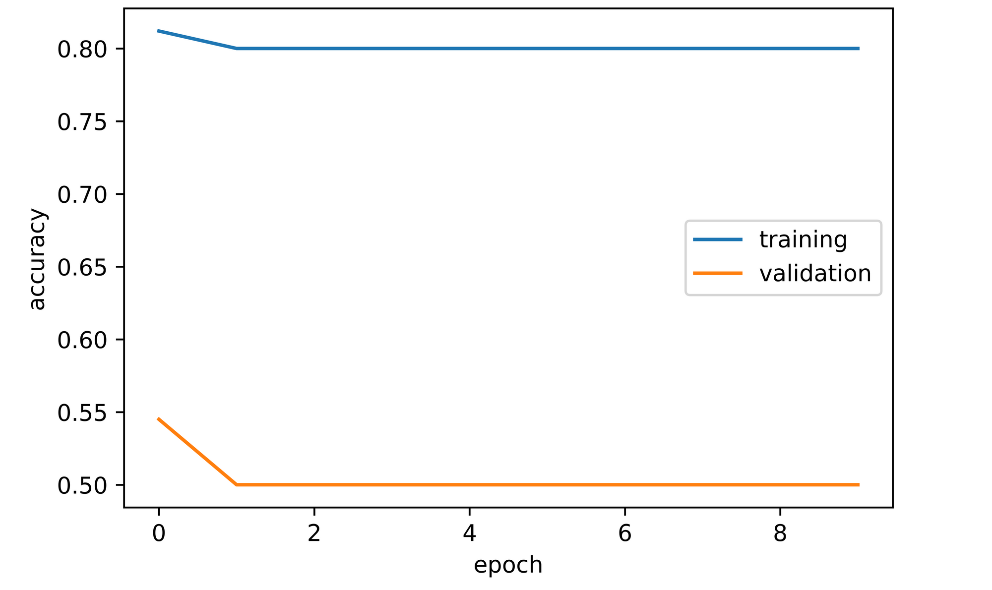
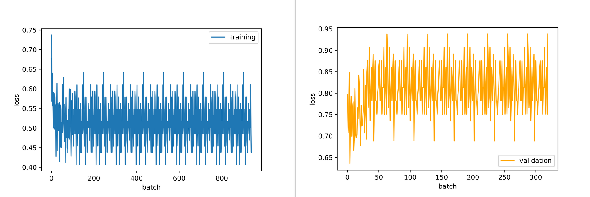
training_set=training_data, validation_set=validation_data)From the results below, turns out a convolutional neural network will do exactly the same thing we did by setting up it's own mock model which classifies every image instance as cat (0) hence a training accuracy of 80% and a validation accuracy of 50%. Just as we logically sought out the easiest way to maximize accuracy/performance on the training set, the optimization process of deep learning/machine learning models have the exact same motivations as they tend to follow the path of least resistance, predicting all images as cats in this case.
Magnitude of the Effect of Class Imbalance on Model Objectives.
As evident from the previous section, class imbalance has an absolutely huge significance on whether a model objective is met or not. It can lure one into a false sense of security as it may yield a high training accuracy as evident in our case where we have a 4:1 imbalance. Based on this premise it is also clear that accuracy does not always tell the full story when it comes to model objectives in classification tasks.
Handling Class Imbalance
There are a number of ways to handle class imbalance in image datasets or any datasets for that matter. In this section we will be looking at 3 of them.
Downsampling
Downsampling refers to the process of reducing the number of instances in the majority class in a bid to match the number of instances in the minority class. For instance in our training data we have 4,800 images of cats and 1,200 images of dogs. If we decide to handle class imbalance via downsampling, we need to reduce the number of cat images to 1,200 as well so we have an equal split between both classes.
This method could lead to a significant reduction in the size of the dataset which might be undesirable in most cases. In our case, if we downsample we would go from a total of 6,000 images to 2,400 images.
Upsampling
Upsampling refers to the process of bringing up the number of instances in the minority class to match the number of instances in the majority class. This could be done by collecting more data instances for the minority class or when that is impossible we could augment the existing data instances by creating modified versions of them.
In our case we would need to increase the number of dog images to 4,800 as well which will bring the size of the dataset to 9,600 instances, up from an original size of 6,000. Upsampling is usually favored over downsampling for this reason as it has the desirable effect of increasing the size of the dataset and in some cases it introduces variation which builds redundancy in trained models.
Utilizing Class Weights
When training a model for classification, implicitly the model places the same importance/weight on all classes and treats them all the same way as regards classification loss. However, we can explicitly place more importance on one class in relation to the other by outrightly specifying how important each class is to us.
The importance we specify is termed class weights, and it can work in our favor in the context of class imbalance. We can place more importance on the minority class thereby forcing the model to learn a mapping that prioritizes identifying that particular class to a certain degree. This will be our focus in the coming section.
Handling Class Imbalance via Class Weights
In this section, we will be attempting to use class weights to adjust the behavior of our model so that it fits as close as possible to our model objective of maximizing recall even as we have an imbalanced dataset. In order to monitor our model objective, we need to modify the convolutional neural network class defined in one of the previous sections to not only calculate accuracy, but to calculate recall and precision as well.
class ConvolutionalNeuralNet_2():
  def __init__(self, network):
    self.network = network.to(device)
    self.optimizer = torch.optim.Adam(self.network.parameters(), lr=1e-3)

  def train(self, loss_function, epochs, batch_size,
            training_set, validation_set):

    #  creating log
    log_dict = {
        'training_loss_per_batch': [],
        'validation_loss_per_batch': [],
        'training_accuracy_per_epoch': [],
        'training_recall_per_epoch': [],
        'training_precision_per_epoch': [],
        'validation_accuracy_per_epoch': [],
        'validation_recall_per_epoch': [],
        'validation_precision_per_epoch': []
    }

    #  defining weight initialization function
    def init_weights(module):
      if isinstance(module, nn.Conv2d):
        torch.nn.init.xavier_uniform_(module.weight)
        module.bias.data.fill_(0.01)
      elif isinstance(module, nn.Linear):
        torch.nn.init.xavier_uniform_(module.weight)
        module.bias.data.fill_(0.01)

    #  defining accuracy function
    def accuracy(network, dataloader):
      network.eval()

      all_predictions = []
      all_labels = []

      #  computing accuracy
      total_correct = 0
      total_instances = 0
      for images, labels in tqdm(dataloader):
        images, labels = images.to(device), labels.to(device)
        all_labels.extend(labels)
        predictions = torch.argmax(network(images), dim=1)
        all_predictions.extend(predictions)
        correct_predictions = sum(predictions==labels).item()
        total_correct+=correct_predictions
        total_instances+=len(images)
      accuracy = round(total_correct/total_instances, 3)

      #  computing recall and precision
      true_positives = 0
      false_negatives = 0
      false_positives = 0
      for idx in range(len(all_predictions)):
        if all_predictions[idx].item()==1 and  all_labels[idx].item()==1:
          true_positives+=1
        elif all_predictions[idx].item()==0 and all_labels[idx].item()==1:
          false_negatives+=1
        elif all_predictions[idx].item()==1 and all_labels[idx].item()==0:
          false_positives+=1
      try:
        recall = round(true_positives/(true_positives + false_negatives), 3)
      except ZeroDivisionError:
        recall = 0.0
      try:
        precision = round(true_positives/(true_positives + false_positives), 3)
      except ZeroDivisionError:
        precision = 0.0
      return accuracy, recall, precision

    #  initializing network weights
    self.network.apply(init_weights)

    #  creating dataloaders
    train_loader = DataLoader(training_set, batch_size)
    val_loader = DataLoader(validation_set, batch_size)

    #  setting convnet to training mode
    self.network.train()

    for epoch in range(epochs):
      print(f'Epoch {epoch+1}/{epochs}')
      train_losses = []

      #  training
      print('training...')
      for images, labels in tqdm(train_loader):
        #  sending data to device
        images, labels = images.to(device), labels.to(device)
        #  resetting gradients
        self.optimizer.zero_grad()
        #  making predictions
        predictions = self.network(images)
        #  computing loss
        loss = loss_function(predictions, labels)
        log_dict['training_loss_per_batch'].append(loss.item())
        train_losses.append(loss.item())
        #  computing gradients
        loss.backward()
        #  updating weights
        self.optimizer.step()
      with torch.no_grad():
        print('deriving training accuracy...')
        #  computing training accuracy
        train_accuracy, train_recall, train_precision = accuracy(self.network, train_loader)
        log_dict['training_accuracy_per_epoch'].append(train_accuracy)
        log_dict['training_recall_per_epoch'].append(train_recall)
        log_dict['training_precision_per_epoch'].append(train_precision)

      #  validation
      print('validating...')
      val_losses = []

      #  setting convnet to evaluation mode
      self.network.eval()

      with torch.no_grad():
        for images, labels in tqdm(val_loader):
          #  sending data to device
          images, labels = images.to(device), labels.to(device)
          #  making predictions
          predictions = self.network(images)
          #  computing loss
          val_loss = loss_function(predictions, labels)
          log_dict['validation_loss_per_batch'].append(val_loss.item())
          val_losses.append(val_loss.item())
        #  computing accuracy
        print('deriving validation accuracy...')
        val_accuracy, val_recall, val_precision = accuracy(self.network, val_loader)
        log_dict['validation_accuracy_per_epoch'].append(val_accuracy)
        log_dict['validation_recall_per_epoch'].append(val_recall)
        log_dict['validation_precision_per_epoch'].append(val_precision)

      train_losses = np.array(train_losses).mean()
      val_losses = np.array(val_losses).mean()

      print(f'training_loss: {round(train_losses, 4)}  training_accuracy: '+
      f'{train_accuracy}  training_recall: {train_recall}  training_precision: {train_precision} *~* validation_loss: {round(val_losses, 4)} '+
      f'validation_accuracy: {val_accuracy}  validation_recall: {val_recall}  validation_precision: {val_precision}\n')

    return log_dict

  def predict(self, x):
return self.network(x)The class weights go into the loss function we decide to use for model training. In this case we have decided to use the cross entropy loss function, and, therefore, the class weights will be defined as a parameter of the loss function eg nn.CrossEntropyLoss(weight=torch.tensor((0.1, 0.9))). The weights take the form (weight of class 0, weight of class 1) and they must both sum to a value of 1.0.
The Other Extreme.
For example, take the code block below, a weight of 0 has been assigned to class 0 and a weight of 1.0 has been assigned to class 1. This implies that we are instructing the model to pay no importance to class 0 hence we expect it to only learn a mapping to class 1. Therefore the model should have an accuracy of 20% since it will only be predicting the minority class and a recall of 100% since there will be no false negative classifications. But with a validation accuracy of 50% it still performs poorly for our objectives.
#  training model
model = ConvolutionalNeuralNet_2(ConvNet())

weight = torch.tensor((0, 1.0))

log_dict = model.train(nn.CrossEntropyLoss(weight=weight), epochs=10, batch_size=64,
                       training_set=training_data, validation_set=validation_data)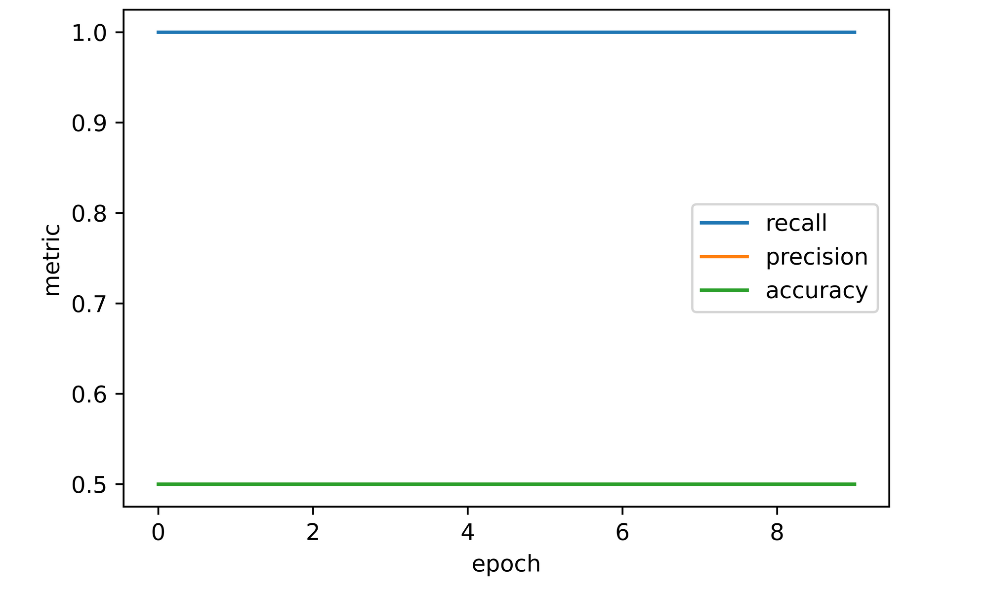
A More Balanced Approach
So just like that we went from a model that would only classify all images as cats to a model that would only classify all images as dogs just by specifying the amount of importance we want to place on each class. Following the same logic, we now know that the best model lies somewhere in-between provided the positive class (1) is still given more priority. Let's try a different combination of weights.
#  training model
model = ConvolutionalNeuralNet_2(ConvNet())

weight = torch.tensor((0.15, 0.85))

log_dict = model.train(nn.CrossEntropyLoss(weight=weight), epochs=10, batch_size=64,
                       training_set=training_data, validation_set=validation_data)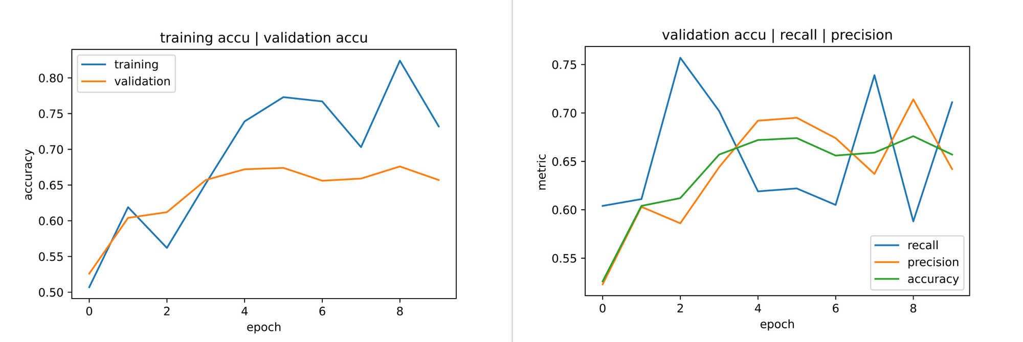
From the plots above it's evident that this combination of weights yield a more balanced model. A validation accuracy of just over 65% was observed by the 10th epoch which implies that the model is not just classifying all images as a either positive or negative, it's actually being discriminative now. Also, at a validation accuracy of 65%, a recall of about 70% was also observed, the best metric combination that fits our model objective we have observed so far.
The Details Lie in Iterations
Just like anything that involves hyperparameter tuning in machine learning, finding the perfect combination of class weights is an involved process which requires a lot of iterations. When that it done then the most optimal combination of class weights can be found.
Note however that using class weights isn't a magic pill to all class imbalance issues. It's possible to use them and not obtain desired results as regards the model objective even when we have their most optimal combination. This will then require the usage of some of the other class imbalance handling methods.
It Goes Beyond Class Imbalance
Sometimes, even when there is no class imbalance, a classification model might still not fit the model objective by default. To illustrate, I trained our convnet on a balanced dataset of cats and dogs (5000 instances in each class) and collected metrics as visualized below.
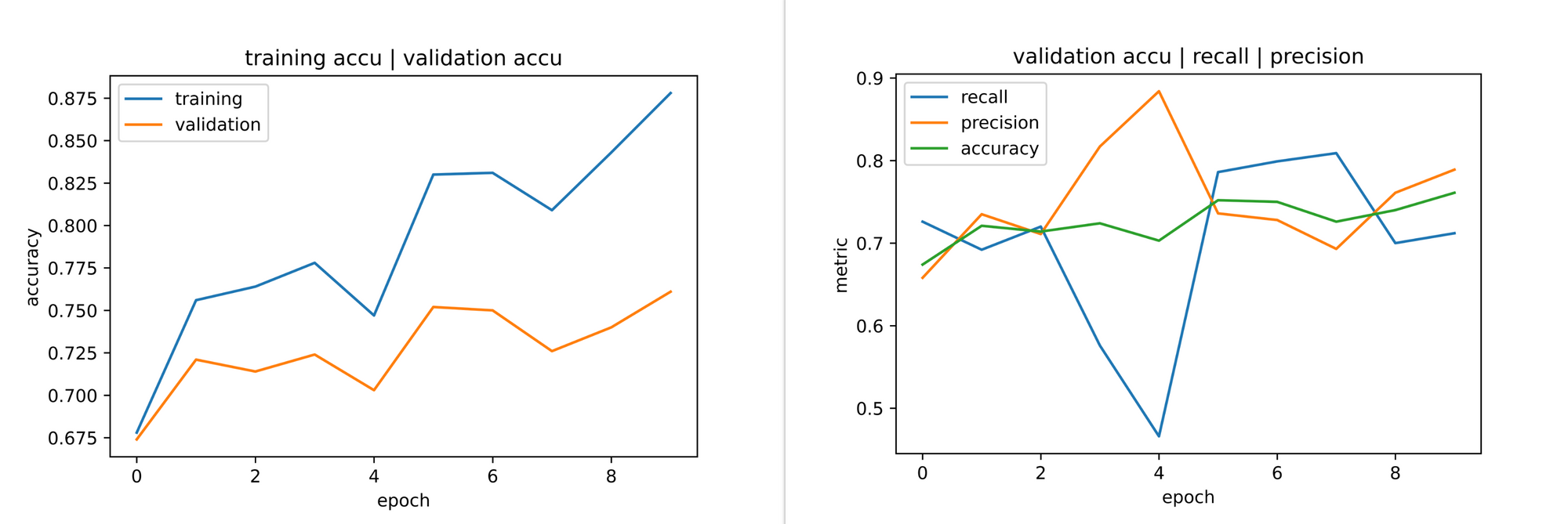
Consider the 5th epoch, even with a validation accuracy of over 70%, validation recall suddenly drops to under 50% which is a big red flag for our model objective as we are trying to maximize recall. Even by the 10th epoch the model doled out more false positive classifications than false negatives (it mistook more cats as dogs more times than it mistook dogs for cats) which is still underwhelming for our model objective. Adjusting class weights will help in this instance to squeeze as much as possible out of validation recall even though the dataset is balanced.
Final Thoughts
In this article, we explored the concept of class imbalance in image datasets. We took a look at the definition of the concept itself and why it may come up in some cases. We also explored the process of defining a clear objective for classification tasks with a view on how more evaluation metrics rather than accuracy can better serve us in meeting our goals. Finally we examined how class imbalance can be tackled whilst taking a keen look at class weights.