
Bring this project to life
A number of factors influence how well a deep learning model generalizes a function or creates a mapping for a specific dataset and a desired objective. In this article, we are going to take a look at what dimensions such as width and depth imply, and examine how they impact the overall performance of convolutional neural network architectures.
#  import dependencies
import torch
import torch.nn as nn
import torch.nn.functional as F
import torchvision
import torchvision.transforms as transforms
import torchvision.datasets as Datasets
from torch.utils.data import Dataset, DataLoader
import numpy as np
import matplotlib.pyplot as plt
import cv2
from tqdm.notebook import tqdm
import seaborn as sns
from torchvision.utils import make_grid
Dimensions
It might sound a bit absurd, but convnets can be thought of as boxes. Just as a box would typically have a width and a depth, the same conventions apply to convnets, as well. In this section we are going to take a look at these dimensions as they relate to convnets.
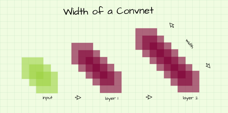
Width
Also known as capacity, the width of a convolutional neural network refers to the number of channels present in its layers. In a typical convnet architecture, the number of channels in each layer increases progressively as we go from one layer to the other, following the same line of thought, this implies that the network gets wider and wider as we go from one layer to the other.
As it regards the impact of width on the performance of a convolutional neural network, at this point we know that each channel in a convolution layer is simply a feature map of extracted features. A convnet with more width (channels per layer) will be able to learn more diverse features from the input image.
In less technical terms, a convnet with more width will be more suited to handling a variety of inputs particularly in a case where classes are somewhat similar. To illustrate, consider a convnet tasked with distinguishing between a sedan and a coupe. These are two classes of cars which look quite similar but for the exception that a sedan has four doors while a coupe has two. In order to learn the subtle differences between both cars it will be beneficial to extract numerous features at each layer so a distinguishing function can be learnt across the network.
While wider convolutional neural networks might be more beneficial, it is imperative to note that the wider the network the higher the number of parameters it possesses. When there are too many parameters, overfitting becomes a very likely possibility.
Consider the two custom convnets architectures below, convnet_2 is wider in comparison to convnet_1 as the number of channels in its layers is much higher. It starts off with 16 channels in layer 1, and terminates at 64 layers in layer 3; while convnet_1 starts off with 8 channels in layer 1, and culminates in 32 layers at layer 3.
class ConvNet_1(nn.Module):
  def __init__(self):
    super().__init__()
    self.conv1 = nn.Conv2d(1, 8, 3, padding=1)
    self.pool1 = nn.MaxPool2d(2)
    self.conv2 = nn.Conv2d(8, 16, 3, padding=1)
    self.pool2 = nn.MaxPool2d(2)
    self.conv3 = nn.Conv2d(16, 32, 3, padding=1)
    self.pool3 = nn.MaxPool2d(2)
    self.conv4 = nn.Conv2d(32, 10, 1)
    self.pool4 = nn.AvgPool2d(3)

  def forward(self, x):
    #-------------
    # INPUT
    #-------------
    x = x.view(-1, 1, 28, 28)

    #-------------
    # LAYER 1
    #-------------
    output_1 = self.conv1(x)
    output_1 = F.relu(output_1)
    output_1 = self.pool1(output_1)

    #-------------
    # LAYER 2
    #-------------
    output_2 = self.conv2(output_1)
    output_2 = F.relu(output_2)
    output_2 = self.pool2(output_2)

    #-------------
    # LAYER 3
    #-------------
    output_3 = self.conv3(output_2)
    output_3 = F.relu(output_3)
    output_3 = self.pool3(output_3)

    #--------------
    # OUTPUT LAYER
    #--------------
    output_4 = self.conv4(output_3)
    output_4 = self.pool4(output_4)
    output_4 = output_4.view(-1, 10)

return torch.sigmoid(output_4)class ConvNet_2(nn.Module):
def __init__(self):
super().__init__()
self.conv1 = nn.Conv2d(1, 16, 3, padding=1)
self.pool1 = nn.MaxPool2d(2)
self.conv2 = nn.Conv2d(16, 32, 3, padding=1)
self.pool2 = nn.MaxPool2d(2)
self.conv3 = nn.Conv2d(32, 64, 3, padding=1)
self.pool3 = nn.MaxPool2d(2)
self.conv4 = nn.Conv2d(64, 10, 1)
self.pool4 = nn.AvgPool2d(3)
def forward(self, x):
#-------------
# INPUT
#-------------
x = x.view(-1, 1, 28, 28)
#-------------
# LAYER 1
#-------------
output_1 = self.conv1(x)
output_1 = F.relu(output_1)
output_1 = self.pool1(output_1)
#-------------
# LAYER 2
#-------------
output_2 = self.conv2(output_1)
output_2 = F.relu(output_2)
output_2 = self.pool2(output_2)
#-------------
# LAYER 3
#-------------
output_3 = self.conv3(output_2)
output_3 = F.relu(output_3)
output_3 = self.pool3(output_3)
#--------------
# OUTPUT LAYER
#--------------
output_4 = self.conv4(output_3)
output_4 = self.pool4(output_4)
output_4 = output_4.view(-1, 10)
return torch.sigmoid(output_4)Depth
The depth of a convolutional neural network refers to the number of layers which it possesses. Depth determines the kind of structures which can be learnt by the convnet.
Typically, shallower layers learn high level features while deeper layers learn low level features. In more technical terms, using a human face for illustration purposes, while the first few layers of the convnet will extract edges pertaining to the overall structure of the face, deeper layers will extract edges pertaining to the eyes, ears, nose, mouth etc.
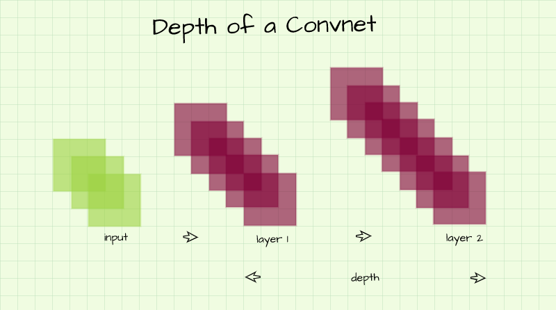
Just as in the case of convnet width, more depth implies more parameters, therefore uncontrolled depth could also result in the network overfitting to the training data. Convnet_3 below is a replica of convnet_1 albeit one with increased depth. Notice that although depth has been increased, the width remains the same as the extra convolution layers have the same number of channels as their preceding layers so the network did not become wider.
class ConvNet_3(nn.Module):
  def __init__(self):
    super().__init__()
    self.conv1 = nn.Conv2d(1, 8, 3, padding=1)
    self.conv2 = nn.Conv2d(8, 8, 3, padding=1)
    self.pool2 = nn.MaxPool2d(2)
    self.conv3 = nn.Conv2d(8, 16, 3, padding=1)
    self.conv4 = nn.Conv2d(16, 16, 3, padding=1)
    self.pool4 = nn.MaxPool2d(2)
    self.conv5 = nn.Conv2d(16, 32, 3, padding=1)
    self.conv6 = nn.Conv2d(32, 32, 3, padding=1)
    self.pool6 = nn.MaxPool2d(2)
    self.conv7 = nn.Conv2d(32, 10, 1)
    self.pool7 = nn.AvgPool2d(3)

  def forward(self, x):
    #-------------
    # INPUT
    #-------------
    x = x.view(-1, 1, 28, 28)

    #-------------
    # LAYER 1
    #-------------
    output_1 = self.conv1(x)
    output_1 = F.relu(output_1)

    #-------------
    # LAYER 2
    #-------------
    output_2 = self.conv2(output_1)
    output_2 = F.relu(output_2)
    output_2 = self.pool2(output_2)

    #-------------
    # LAYER 3
    #-------------
    output_3 = self.conv3(output_2)
    output_3 = F.relu(output_3)

    #-------------
    # LAYER 4
    #-------------
    output_4 = self.conv4(output_3)
    output_4 = F.relu(output_4)
    output_4 = self.pool4(output_4)

    #-------------
    # LAYER 5
    #-------------
    output_5 = self.conv5(output_4)
    output_5 = F.relu(output_5)

    #-------------
    # LAYER 6
    #-------------
    output_6 = self.conv6(output_5)
    output_6 = F.relu(output_6)
    output_6 = self.pool6(output_6)

    #--------------
    # OUTPUT LAYER
    #--------------
    output_7 = self.conv7(output_6)
    output_7 = self.pool7(output_7)
    output_7 = output_7.view(-1, 10)

return torch.sigmoid(output_7)Benchmarking Convnet Performance Based on Dimensions
In this section, we are going to compare convnet performances based on width and depth. Convnet_1 will be used as a baseline while convnet_2 will serve as a version of convnet_1 with increased width and convnet_3 will serve as a version with increased depth. Convnet_4 below combines both the increased width and depth seen in convnet_2 and 3 respectively.
class ConvNet_4(nn.Module):
  def __init__(self):
    super().__init__()
    self.conv1 = nn.Conv2d(1, 16, 3, padding=1)
    self.conv2 = nn.Conv2d(16, 16, 3, padding=1)
    self.pool2 = nn.MaxPool2d(2)
    self.conv3 = nn.Conv2d(16, 32, 3, padding=1)
    self.conv4 = nn.Conv2d(32, 32, 3, padding=1)
    self.pool4 = nn.MaxPool2d(2)
    self.conv5 = nn.Conv2d(32, 64, 3, padding=1)
    self.conv6 = nn.Conv2d(64, 64, 3, padding=1)
    self.pool6 = nn.MaxPool2d(2)
    self.conv7 = nn.Conv2d(64, 10, 1)
    self.pool7 = nn.AvgPool2d(3)

  def forward(self, x):
    #-------------
    # INPUT
    #-------------
    x = x.view(-1, 1, 28, 28)

    #-------------
    # LAYER 1
    #-------------
    output_1 = self.conv1(x)
    output_1 = F.relu(output_1)

    #-------------
    # LAYER 2
    #-------------
    output_2 = self.conv2(output_1)
    output_2 = F.relu(output_2)
    output_2 = self.pool2(output_2)

    #-------------
    # LAYER 3
    #-------------
    output_3 = self.conv3(output_2)
    output_3 = F.relu(output_3)

    #-------------
    # LAYER 4
    #-------------
    output_4 = self.conv4(output_3)
    output_4 = F.relu(output_4)
    output_4 = self.pool4(output_4)

    #-------------
    # LAYER 5
    #-------------
    output_5 = self.conv5(output_4)
    output_5 = F.relu(output_5)

    #-------------
    # LAYER 6
    #-------------
    output_6 = self.conv6(output_5)
    output_6 = F.relu(output_6)
    output_6 = self.pool6(output_6)

    #--------------
    # OUTPUT LAYER
    #--------------
    output_7 = self.conv7(output_6)
    output_7 = self.pool7(output_7)
    output_7 = output_7.view(-1, 10)

    return torch.sigmoid(output_7)
Benchmark Dataset: FashionMNIST
The FashionMNIST dataset will be used for our benchmarking objective. This is a dataset containing 28 pixel x 28 pixel images of common fashion accessories such as pullovers, bags, shirts, dresses and so on. This dataset comes preloaded PyTorch and can be imported as such:
#  laoding training data
training_set = Datasets.FashionMNIST(root='./', download=True,
                                      transform=transforms.ToTensor())

#  loading validation data
validation_set = Datasets.FashionMNIST(root='./', download=True, train=False,
                                        transform=transforms.ToTensor())
In order to visualize the dataset, let's quickly create a dataloader and then extract the images from one batch for visualization. Note: there's probably a better way to do this, if you find one you should follow it, I chose to do it this way out of habit.
val_loader = DataLoader(validation_set, 32)

for images, labels in val_loader:
  print(images.shape)
  break

#  visualising images
plt.figure(dpi=150)
plt.title('images')
plt.imshow(np.transpose(make_grid(images, padding=4, normalize=True),
                        (1,2,0)))
plt.axis('off')
plt.savefig('fmnist.png', dpi=1000)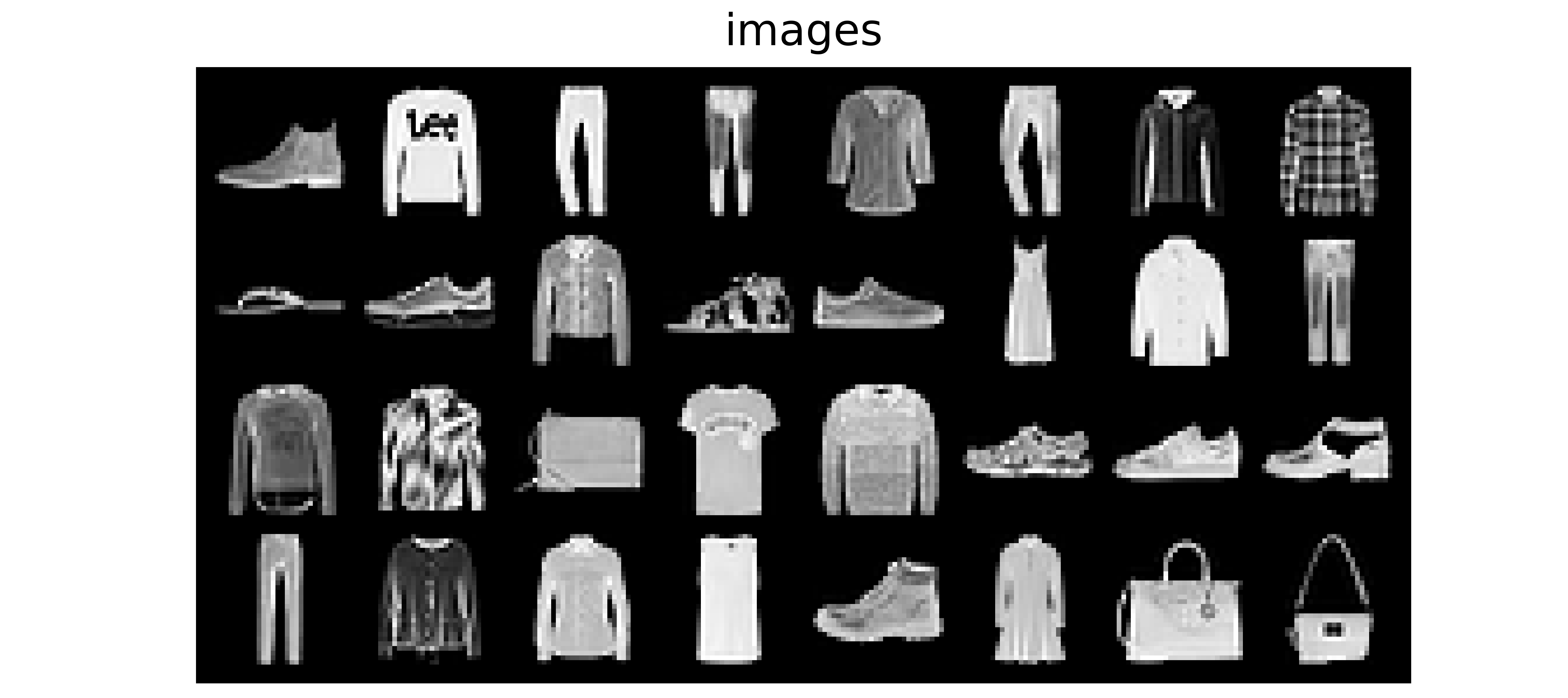
| Label | Description |
|---|---|
| 0 | T-Shirt |
| 1 | Trouser |
| 2 | Pullover |
| 3 | Dress |
| 4 | Coat |
| 5 | Sandal |
| 6 | Shirt |
| 7 | Sneaker |
| 8 | Bag |
| 9 | Ankle boot |
Convolutional Neural Network Class
Bring this project to life
In order to train and make use of our convnets, let's define a class which will encompass training and prediction as seen in the code block below. The train() method takes in parameters such as the loss function, number of epochs to train for, batch size, training set and validation set.
From the training and validation sets, dataloaders are created within the function itself. This is done so as to allow for the possibility of changing batch sizes when instantiating a member of the class. Notice that the data in the dataloaders are not shuffled or sampled at random, this is to allow for uniformity of training, which is imperative when comparing several models as we are about to do.
Additionally, two inner functions are defined within the train() method, they are init_weights() and accuracy(). Init_weights() serves the purpose of ensuring that the weights of all models to be compared are initialized the same way which will again allow for uniformity of training. Apart from that, it's also a measure which could allow neural networks train faster. The accuracy() function does exactly what its name implies, it computes the accuracy of a convnet.
#  setup device
if torch.cuda.is_available():
  device = torch.device('cuda:0')
  print('Running on the GPU')
else:
  device = torch.device('cpu')
  print('Running on the CPU')
class ConvolutionalNeuralNet():
def __init__(self, network):
self.network = network.to(device)
self.optimizer = torch.optim.Adam(self.network.parameters(), lr=3e-4)
def train(self, loss_function, epochs, batch_size,
training_set, validation_set):
# creating log
log_dict = {
'training_loss_per_batch': [],
'validation_loss_per_batch': [],
'training_accuracy_per_epoch': [],
'validation_accuracy_per_epoch': []
}
# defining weight initialization function
def init_weights(module):
if isinstance(module, nn.Conv2d):
torch.nn.init.xavier_uniform_(module.weight)
module.bias.data.fill_(0.01)
# defining accuracy function
def accuracy(network, dataloader):
total_correct = 0
total_instances = 0
for images, labels in tqdm(dataloader):
images, labels = images.to(device), labels.to(device)
predictions = torch.argmax(network(images), dim=1)
correct_predictions = sum(predictions==labels).item()
total_correct+=correct_predictions
total_instances+=len(images)
return round(total_correct/total_instances, 3)
# initializing network weights
self.network.apply(init_weights)
# creating dataloaders
train_loader = DataLoader(training_set, batch_size)
val_loader = DataLoader(validation_set, batch_size)
for epoch in range(epochs):
print(f'Epoch {epoch+1}/{epochs}')
train_losses = []
# training
print('training...')
for images, labels in tqdm(train_loader):
# sending data to device
images, labels = images.to(device), labels.to(device)
# resetting gradients
self.optimizer.zero_grad()
# making predictions
predictions = self.network(images)
# computing loss
loss = loss_function(predictions, labels)
log_dict['training_loss_per_batch'].append(loss.item())
train_losses.append(loss.item())
# computing gradients
loss.backward()
# updating weights
self.optimizer.step()
with torch.no_grad():
print('deriving training accuracy...')
# computing training accuracy
train_accuracy = accuracy(self.network, train_loader)
log_dict['training_accuracy_per_epoch'].append(train_accuracy)
# validation
print('validating...')
val_losses = []
with torch.no_grad():
for images, labels in tqdm(val_loader):
# sending data to device
images, labels = images.to(device), labels.to(device)
# making predictions
predictions = self.network(images)
# computing loss
val_loss = loss_function(predictions, labels)
log_dict['validation_loss_per_batch'].append(val_loss.item())
val_losses.append(val_loss.item())
# computing accuracy
print('deriving validation accuracy...')
val_accuracy = accuracy(self.network, val_loader)
log_dict['validation_accuracy_per_epoch'].append(val_accuracy)
train_losses = np.array(train_losses).mean()
val_losses = np.array(val_losses).mean()
print(f'training_loss: {round(train_losses, 4)} training_accuracy: '+
f'{train_accuracy} validation_loss: {round(val_losses, 4)} '+
f'validation_accuracy: {val_accuracy}\n')
return log_dict
def predict(self, x):
return self.network(x) Benchmark Results
ConvNet_1
Again remember that convnet_1 serves as the baseline for this benchmarking task. Let's instantiate convnet_1 as a member of the ConvolutionalNeuralNet class using the cross entropy loss function and a batch size of 64 then train it for 10 epochs as seen below.
#  instantiating convnet_1
model_1 = ConvolutionalNeuralNet(ConvNet_1())

#  training convnet_1
log_dict_1 = model_1.train(nn.CrossEntropyLoss(), epochs=10, batch_size=64,
                           training_set=training_set, validation_set=validation_set)
From the log obtained we can see that overall, both training and validation accuracy were on an upward trend throughout training with training accuracy being higher than validation accuracy. The convnet attained a validation accuracy of approximately 54% after just one epoch of training and continued to rise steadily until it terminated at just under 68% by the tenth epoch.
#  visualizing accuracies
sns.lineplot(y=log_dict_1['training_accuracy_per_epoch'], x=range(len(log_dict_1['training_accuracy_per_epoch'])), label='training')

sns.lineplot(y=log_dict_1['validation_accuracy_per_epoch'], x=range(len(log_dict_1['validation_accuracy_per_epoch'])), label='validation')

plt.xlabel('epoch')
plt.ylabel('accuracy')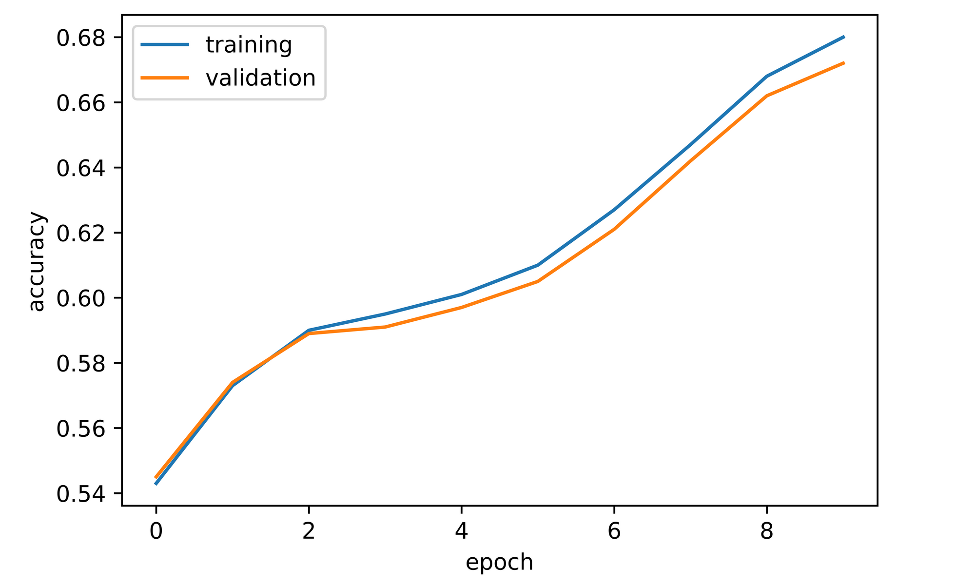
ConvNet_2
Convnet_2 is a version of convnet_1 with increased width. Essentially, convnet_2 is twice as wide as convnet_1 with the same number of layer. Keeping all parameters the same, let's train convnet_2 for 10 epochs and visualize the results.
#  instantiating convnet_2
model_2 = ConvolutionalNeuralNet(ConvNet_2())

#  training convnet_2
log_dict_2 = model_2.train(nn.CrossEntropyLoss(), epochs=10, batch_size=64,
                           training_set=training_set, validation_set=validation_set)
Overall, both training and validation accuracy increased throughout the course of training. Validation accuracy was about 62% after just one epoch, 8% higher than convnet_1 at the same instance. Validation accuracy did dip to just under 60% by the second epoch but it recovered and continued to increase to a zenith of just under 72% by epoch 10, about 5% higher than convnet_1 at that point.
#  visualizing accuracies
sns.lineplot(y=log_dict_2['training_accuracy_per_epoch'], x=range(len(log_dict_2['training_accuracy_per_epoch'])), label='training')

sns.lineplot(y=log_dict_2['validation_accuracy_per_epoch'], x=range(len(log_dict_2['validation_accuracy_per_epoch'])), label='validation')

plt.xlabel('epoch')
plt.ylabel('accuracy')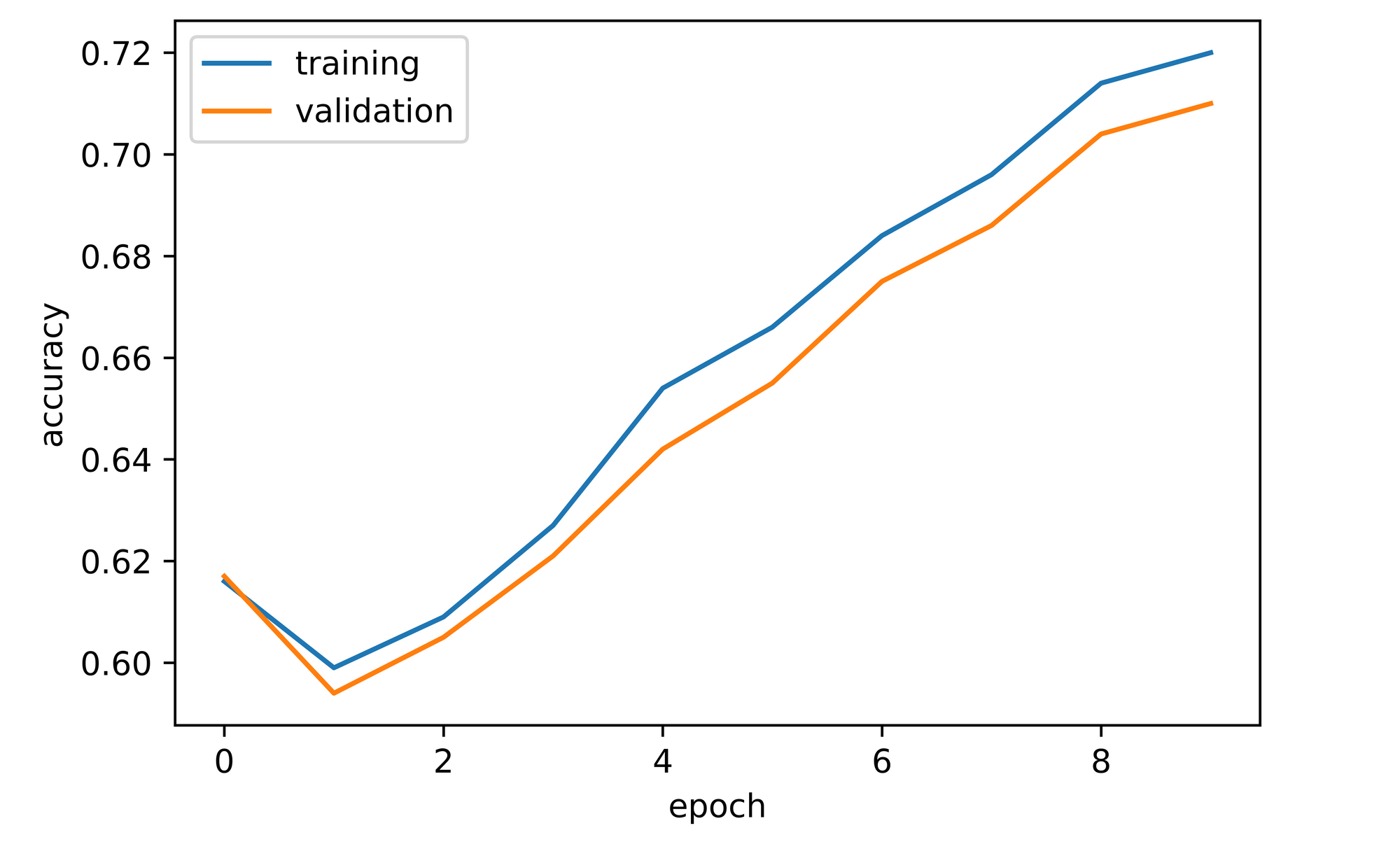
ConvNet_3
Convnet_3 is a version of convnet_1 with increased depth. Essentially it twice as deep but with the same width. Keeping all parameters equal, let's train convnet_3 for 10 epochs and explore the results.
#  instantiating convnet_3
model_3 = ConvolutionalNeuralNet(ConvNet_3())

#  training convnet_3
log_dict_3 = model_3.train(nn.CrossEntropyLoss(), epochs=10, batch_size=64,
                           training_set=training_set, validation_set=validation_set)
Just like the previous two convnets, an overall increase in both training and validation accuracies was observed throughout the course of model training. Validation accuracy attained after one epoch was about 49%, significantly lower than convnet_1 by five percentage points at the same stage. Performance however rebounded and increased sharply to about 72% by the third epoch after which it fluctuated before eventually settling at just under 80% by epoch 10, completely eclipsing convnet_1's performance.
#  visualizing accuracies
sns.lineplot(y=log_dict_3['training_accuracy_per_epoch'], x=range(len(log_dict_3['training_accuracy_per_epoch'])), label='training')

sns.lineplot(y=log_dict_3['validation_accuracy_per_epoch'], x=range(len(log_dict_3['validation_accuracy_per_epoch'])), label='validation')

plt.xlabel('epoch')
plt.ylabel('accuracy')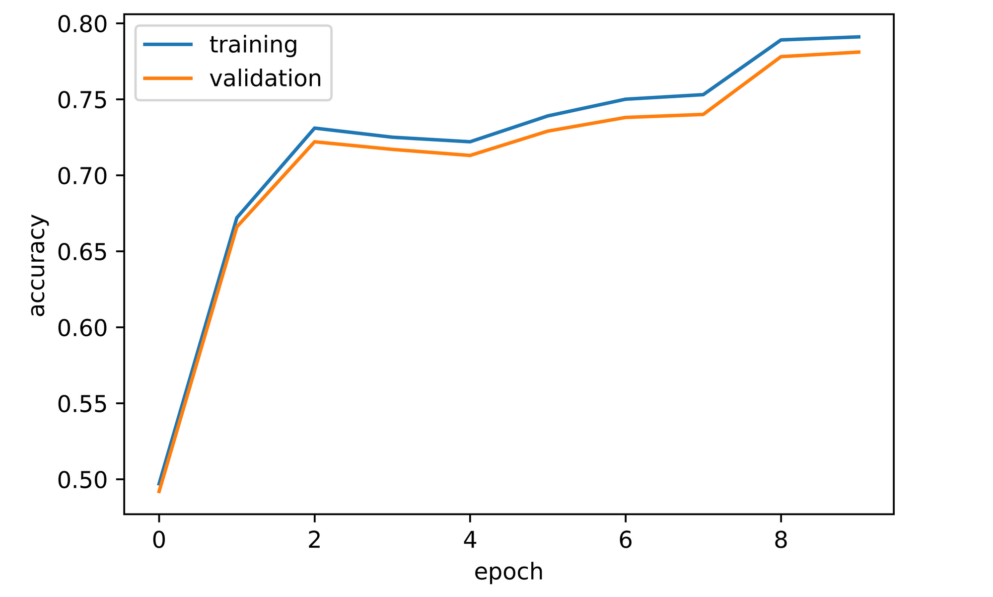
ConvNet_4
Convnet_4 is a version of convnet_1 with increased depth and width. Essentially it is twice as wide while also being twice as deep. Keeping all parameters the same, let's train convnet_4 for 10 epochs and summarize its results.
#  instantiating convnet_4
model_4 = ConvolutionalNeuralNet(ConvNet_4())

#  training convnet_4
log_dict_4 = model_4.train(nn.CrossEntropyLoss(), epochs=10, batch_size=64,
                           training_set=training_set, validation_set=validation_set)
Overall, both training and validation accuracy increased over the course of model training. Validation accuracy attained after the first epoch stood at approximately 62%, seven percentage points higher than convnet_1. From the second epoch up to the forth, validation accuracy increased markedly to a value of just under 76%, it then increased slightly before dipping and then increasing to just under 78%.
#  visualizing accuracies
sns.lineplot(y=log_dict_4['training_accuracy_per_epoch'], x=range(len(log_dict_4['training_accuracy_per_epoch'])), label='training')

sns.lineplot(y=log_dict_4['validation_accuracy_per_epoch'], x=range(len(log_dict_4['validation_accuracy_per_epoch'])), label='validation')

plt.xlabel('epoch')
plt.ylabel('accuracy')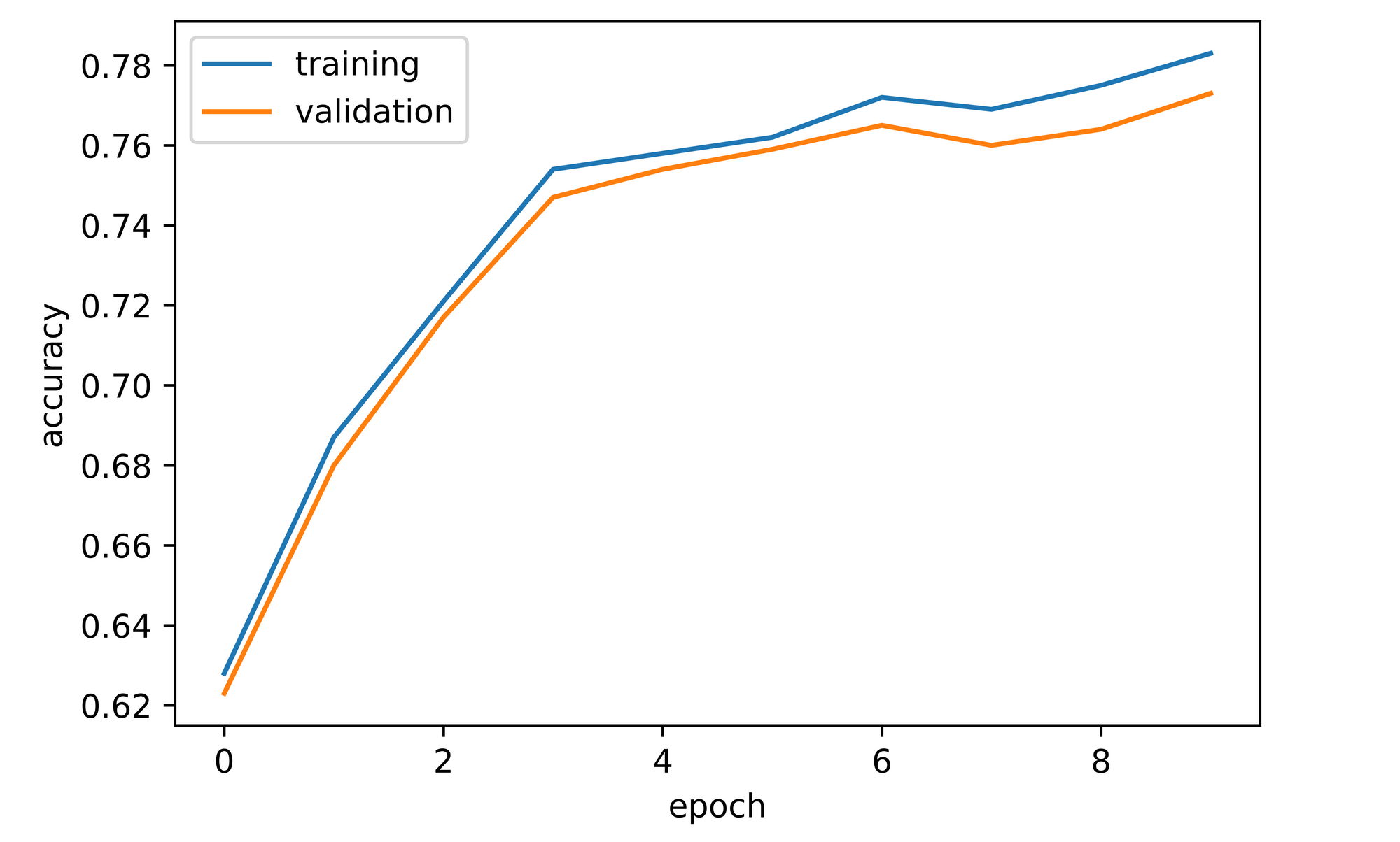
Comparing Performance
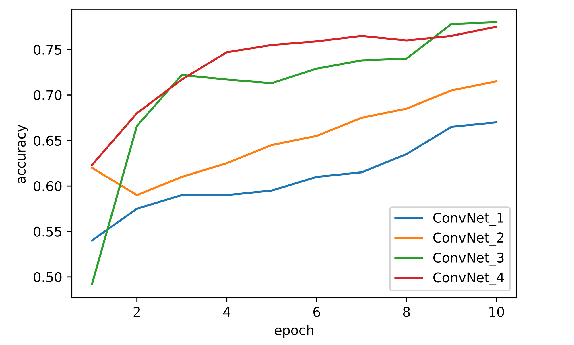
Comparing performance across all four convnets, we can infer that increasing dimensions has a positive correlation with model performance. In all cases where at least one dimension is increased a significant jump in convnet performance is observed.
| Baseline | Increased Width (x2) | Increased Depth (x2) | Increased Depth (x2) & Width (x2) |
|---|---|---|---|
| 54.0 | 62.0 | 49.0 | 62.0 |
| 57.5 | 59.0 | 66.5 | 68.0 |
| 59.0 | 61.0 | 72.0 | 71.5 |
| 59.0 | 62.5 | 71.5 | 74.5 |
| 59.5 | 64.5 | 71.0 | 75.5 |
| 61.0 | 65.5 | 73.0 | 76.0 |
| 61.5 | 67.5 | 74.0 | 76.5 |
| 63.5 | 68.5 | 74.0 | 76.0 |
| 66.5 | 70.5 | 78.0 | 76.5 |
| 67.0 | 71.5 | 78.0 | 77.5 |
| ConvNet_1 | ConvNet_2 | ConvNet_3 | ConvNet_4 |
All Units are in Percentage (%)
Overall, convnet_3 (increased depth) seems to have outperformed all other convnets with convnet_4 (increased depth and width) coming a close second. Convnet_2 (increased width) comes a distant third while the baseline convnet_1 performed the worst out of all four. It should be noted however that the convnets were only trained for 10 epochs, to derive more conclusive results they should all be trained to optimal performance.
Final Remarks
In this article, we explored what dimensions imply in a convolutional neural network context. We created a custom convnet architecture as a baseline model then proceeded to create versions of it, one with increased width, another with increased depth and the last one with both increased depth and width.
All four convents were trained on the FashionMNIST dataset so as to benchmark them against one another. From the results obtained, it was seen that the best performance came when depth was increased while the worst performance was observed from the baseline model. These results infer that a convolutional neural network's dimensions do in fact play a vital role in how well the convnet will perform.