
Bring this project to life
Often times, deep learning models are said to be black boxed in nature. Black boxed in the sense that their outputs are difficult to explain or some times simply unexplainable. However, there are some Python libraries which help to provide some sort of explanation to the output of deep learning models. In this article, we will be taking a look at one of those libraries: SHAP.
#  article dependencies
import torch
import torch.nn as nn
import torch.nn.functional as F
import torchvision
import torchvision.transforms as transforms
import torchvision.datasets as Datasets
from torch.utils.data import Dataset, DataLoader
import numpy as np
import matplotlib.pyplot as plt
import cv2
from tqdm.notebook import tqdm
import seaborn as sns
from torchvision.utils import make_grid
!pip install shap
import shap
if torch.cuda.is_available():
device = torch.device('cuda:0')
print('Running on the GPU')
else:
device = torch.device('cpu')
print('Running on the CPU')Model Explainability
Model explainability refers to the process whereby outputs produced by machine learning models are explained in terms of how and which features influence the model's actual output. For instance, consider a random forest model trained to predict house prices; assume that dataset the model was trained on only has 3 features, number of bedrooms, number of bathrooms and size of the living room. Assume the model predicts a house to be worth about $300,000, with model explainability we can derive insights on how much each feature contributes either positively or negatively to the predicted price.
Model Explainability in the Context of Computer Vision
As regards deep learning, computer vision classification tasks in particular, since features are essentially pixels, model explainability helps to identify pixels which contribute negatively or positively to the predicted class.
In this article, the SHAP library will be used for deep learning model explainability. SHAP, short for Shapely Additive exPlanations is a game theory based approach to explaining outputs of machine learning models, more information can be found in its official documentation.
Implementing Deep Learning Model Explainability
In this section, we will be training a convolutional neural network for a classification task before proceeding to derive a insight into why the model classifies an instance of data into a specific class using the SHAP library.
Dataset
The dataset to be used for training purposes as regards this article will be the CIFAR10 dataset. This is a dataset containing 32 x 32 pixel images belonging to 10 distinct classes ranging from airplanes to horses. It can be loaded in PyTorch using the code cell below.
#  loading training data
training_set = Datasets.CIFAR10(root='./', download=True,
                                transform=transforms.ToTensor())

#  loading validation data
validation_set = Datasets.CIFAR10(root='./', download=True, train=False,
                                  transform=transforms.ToTensor())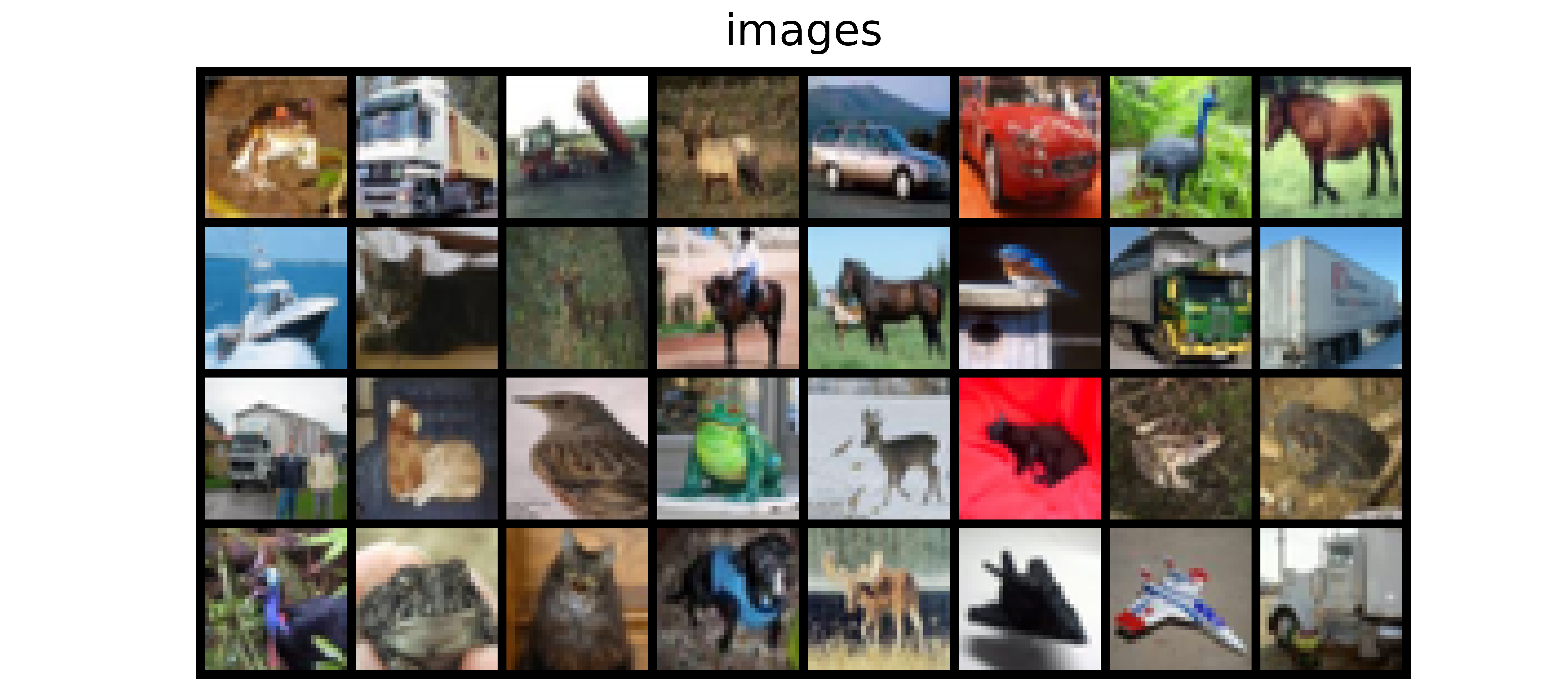
| Label | Description |
|---|---|
| 0 | Airplane |
| 1 | Automobile |
| 2 | Bird |
| 3 | Cat |
| 4 | Deer |
| 5 | Dog |
| 6 | Frog |
| 7 | Horse |
| 8 | Ship |
| 9 | Truck |
Model Architecture
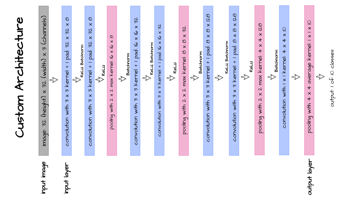
The model architecture as illustrated above is implemented in the following code cell. This is a custom architecture designed purposefully for the sake of this article. This architecture takes in 32 x 32 pixel images and is comprised of 7 convolutional layers.
class ConvNet(nn.Module):
  def __init__(self):
    super().__init__()
    self.conv1 = nn.Conv2d(3, 8, 3, padding=1)
    self.batchnorm1 = nn.BatchNorm2d(8)
    self.conv2 = nn.Conv2d(8, 8, 3, padding=1)
    self.batchnorm2 = nn.BatchNorm2d(8)
    self.pool2 = nn.MaxPool2d(2)
    self.conv3 = nn.Conv2d(8, 32, 3, padding=1)
    self.batchnorm3 = nn.BatchNorm2d(32)
    self.conv4 = nn.Conv2d(32, 32, 3, padding=1)
    self.batchnorm4 = nn.BatchNorm2d(32)
    self.pool4 = nn.MaxPool2d(2)
    self.conv5 = nn.Conv2d(32, 128, 3, padding=1)
    self.batchnorm5 = nn.BatchNorm2d(128)
    self.conv6 = nn.Conv2d(128, 128, 3, padding=1)
    self.batchnorm6 = nn.BatchNorm2d(128)
    self.pool6 = nn.MaxPool2d(2)
    self.conv7 = nn.Conv2d(128, 10, 1)
    self.pool7 = nn.AvgPool2d(3)

  def forward(self, x):
    #-------------
    # INPUT
    #-------------
    x = x.view(-1, 3, 32, 32)

    #-------------
    # LAYER 1
    #-------------
    output_1 = self.conv1(x)
    output_1 = F.relu(output_1)
    output_1 = self.batchnorm1(output_1)

    #-------------
    # LAYER 2
    #-------------
    output_2 = self.conv2(output_1)
    output_2 = F.relu(output_2)
    output_2 = self.pool2(output_2)
    output_2 = self.batchnorm2(output_2)

    #-------------
    # LAYER 3
    #-------------
    output_3 = self.conv3(output_2)
    output_3 = F.relu(output_3)
    output_3 = self.batchnorm3(output_3)

    #-------------
    # LAYER 4
    #-------------
    output_4 = self.conv4(output_3)
    output_4 = F.relu(output_4)
    output_4 = self.pool4(output_4)
    output_4 = self.batchnorm4(output_4)

    #-------------
    # LAYER 5
    #-------------
    output_5 = self.conv5(output_4)
    output_5 = F.relu(output_5)
    output_5 = self.batchnorm5(output_5)

    #-------------
    # LAYER 6
    #-------------
    output_6 = self.conv6(output_5)
    output_6 = F.relu(output_6)
    output_6 = self.pool6(output_6)
    output_6 = self.batchnorm6(output_6)

    #--------------
    # OUTPUT LAYER
    #--------------
    output_7 = self.conv7(output_6)
    output_7 = self.pool7(output_7)
    output_7 = output_7.view(-1, 10)

    return F.softmax(output_7, dim=1)
Convolutional Neural Network Class
In order to neatly put together our model, we will write a class which encompasses both training, validation and model utilization into one object as seen below.
class ConvolutionalNeuralNet():
  def __init__(self, network):
    self.network = network.to(device)
    self.optimizer = torch.optim.Adam(self.network.parameters(), lr=1e-3)

  def train(self, loss_function, epochs, batch_size,
            training_set, validation_set):

    #  creating log
    log_dict = {
        'training_loss_per_batch': [],
        'validation_loss_per_batch': [],
        'training_accuracy_per_epoch': [],
        'training_recall_per_epoch': [],
        'training_precision_per_epoch': [],
        'validation_accuracy_per_epoch': [],
        'validation_recall_per_epoch': [],
        'validation_precision_per_epoch': []
    }

    #  defining weight initialization function
    def init_weights(module):
      if isinstance(module, nn.Conv2d):
        torch.nn.init.xavier_uniform_(module.weight)
        module.bias.data.fill_(0.01)
      elif isinstance(module, nn.Linear):
        torch.nn.init.xavier_uniform_(module.weight)
        module.bias.data.fill_(0.01)

    #  defining accuracy function
    def accuracy(network, dataloader):
      network.eval()

      all_predictions = []
      all_labels = []

      #  computing accuracy
      total_correct = 0
      total_instances = 0
      for images, labels in tqdm(dataloader):
        images, labels = images.to(device), labels.to(device)
        all_labels.extend(labels)
        predictions = torch.argmax(network(images), dim=1)
        all_predictions.extend(predictions)
        correct_predictions = sum(predictions==labels).item()
        total_correct+=correct_predictions
        total_instances+=len(images)
      accuracy = round(total_correct/total_instances, 3)

      #  computing recall and precision
      true_positives = 0
      false_negatives = 0
      false_positives = 0
      for idx in range(len(all_predictions)):
        if all_predictions[idx].item()==1 and  all_labels[idx].item()==1:
          true_positives+=1
        elif all_predictions[idx].item()==0 and all_labels[idx].item()==1:
          false_negatives+=1
        elif all_predictions[idx].item()==1 and all_labels[idx].item()==0:
          false_positives+=1
      try:
        recall = round(true_positives/(true_positives + false_negatives), 3)
      except ZeroDivisionError:
        recall = 0.0
      try:
        precision = round(true_positives/(true_positives + false_positives), 3)
      except ZeroDivisionError:
        precision = 0.0
      return accuracy, recall, precision

    #  initializing network weights
    self.network.apply(init_weights)

    #  creating dataloaders
    train_loader = DataLoader(training_set, batch_size)
    val_loader = DataLoader(validation_set, batch_size)

    #  setting convnet to training mode
    self.network.train()

    for epoch in range(epochs):
      print(f'Epoch {epoch+1}/{epochs}')
      train_losses = []

      #  training
      print('training...')
      for images, labels in tqdm(train_loader):
        #  sending data to device
        images, labels = images.to(device), labels.to(device)
        #  resetting gradients
        self.optimizer.zero_grad()
        #  making predictions
        predictions = self.network(images)
        #  computing loss
        loss = loss_function(predictions, labels)
        log_dict['training_loss_per_batch'].append(loss.item())
        train_losses.append(loss.item())
        #  computing gradients
        loss.backward()
        #  updating weights
        self.optimizer.step()
      with torch.no_grad():
        print('deriving training accuracy...')
        #  computing training accuracy
        train_accuracy, train_recall, train_precision = accuracy(self.network, train_loader)
        log_dict['training_accuracy_per_epoch'].append(train_accuracy)
        log_dict['training_recall_per_epoch'].append(train_recall)
        log_dict['training_precision_per_epoch'].append(train_precision)

      #  validation
      print('validating...')
      val_losses = []

      #  setting convnet to evaluation mode
      self.network.eval()

      with torch.no_grad():
        for images, labels in tqdm(val_loader):
          #  sending data to device
          images, labels = images.to(device), labels.to(device)
          #  making predictions
          predictions = self.network(images)
          #  computing loss
          val_loss = loss_function(predictions, labels)
          log_dict['validation_loss_per_batch'].append(val_loss.item())
          val_losses.append(val_loss.item())
        #  computing accuracy
        print('deriving validation accuracy...')
        val_accuracy, val_recall, val_precision = accuracy(self.network, val_loader)
        log_dict['validation_accuracy_per_epoch'].append(val_accuracy)
        log_dict['validation_recall_per_epoch'].append(val_recall)
        log_dict['validation_precision_per_epoch'].append(val_precision)

      train_losses = np.array(train_losses).mean()
      val_losses = np.array(val_losses).mean()

      print(f'training_loss: {round(train_losses, 4)}  training_accuracy: '+
      f'{train_accuracy}  training_recall: {train_recall}  training_precision: {train_precision} *~* validation_loss: {round(val_losses, 4)} '+
      f'validation_accuracy: {val_accuracy}  validation_recall: {val_recall}  validation_precision: {val_precision}\n')

    return log_dict

  def predict(self, x):
    return self.network(x)
Model Training
Bring this project to life
With everything setup, it's now time to train the model. Using parameters as defined, the model is trained for 15 epochs.
model = ConvolutionalNeuralNet(ConvNet())
log_dict = model.train(nn.CrossEntropyLoss(), epochs=15, batch_size=64,
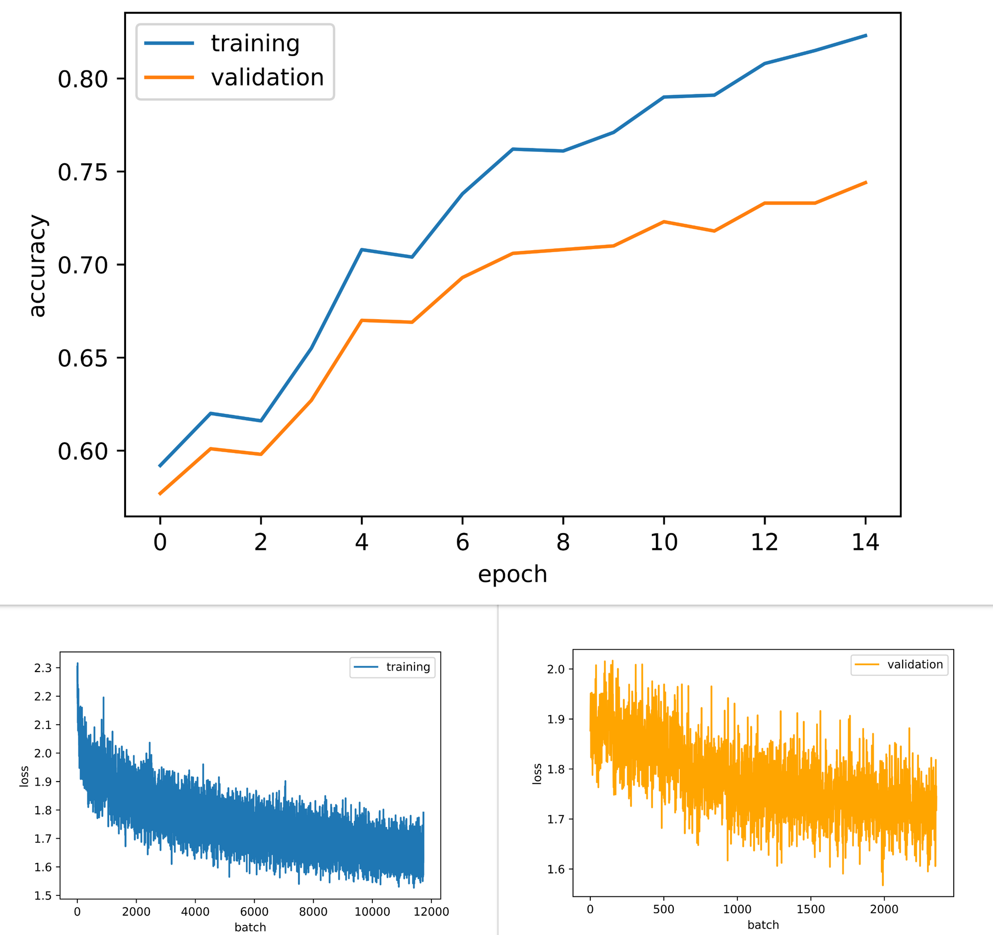
training_set=training_set, validation_set=validation_set)From results obtained, both training and validation accuracy increased through the course of model training. Validation accuracy attained a value just under 75%, not the best performing model but will suffice for this article's objectives. Furthermore, both training and validation losses are down-trending indicative of better performance being obtained with more epochs of training.
Model Explainability
In this section we will be attempting to explain/derive insights into the classifications made by the model trained in the previous section. As mentioned previously, we will be using the SHAP library for this purpose.
Basically, the library does this by utilizing the model in classifying a couple of instances in a bid to understand its behavior and the nature of its outputs, this 'understanding' is called the explainer. Afterwards, using the object containing the explainer, values are then assigned to each feature (pixels in this case) which influences the classification made by the model, these values are termed SHAP values. These SHAP values are the actual metrics which imply explainability; based on the magnitude of these values one can develop an idea into how each pertinent feature has contributed to the classification made by the model. Finally, a plot called a SHAP plot is produced to make interpretation of the aforementioned values easier.
Creating a Mask
As mentioned previously, in order to generate SHAP values an explainer has to have been generated prior. This explainer makes classification on some data instances, these data instances are called a mask. For this article, the first 200 instances in the validation set are selected as the mask. There are thereafter converted into a PyTorch dataset by instantiating them as a member of the CustomMask class.
#  defining dataset class
class CustomMask(Dataset):
  def __init__(self, data, transforms=None):
    self.data = data
    self.transforms = transforms

  def __len__(self):
    return len(self.data)

  def __getitem__(self, idx):
    image = self.data[idx]

    if self.transforms!=None:
      image = self.transforms(image)
    return image

#  creating explainer mask
mask = validation_set.data[:200]

#  turning mask to pytorch dataset
mask = CustomMask(mask, transforms=transforms.ToTensor())
Explainability Function
All the steps outlined above can then be put together to produce a function which implements model explainability by producing SHAP plots for any instance of data classified by the model.
The function below does specifically that. Firstly, it takes in parameters such as an image in array form, a mask and a deep learning model. Next the image array is converted to a tensor and classification is made before mapping the classification vector output to a dictionary of labels native to CIFAR10.
Thereafter, an explainer is derived from the mask and model supplied before SHAP values are produced for the image of choice using this explainer. A SHAP plot is then returned for easy interpretation.
def plot_shap(image_array, mask, model):
  """
  This function performs model explainability
  by producing shap plots for a data instance
  """
  #  converting image to tensor
  image = transforms.ToTensor()(image_array)
  image = image.to(device)

  #-----------------
  #  CLASSIFICATION
  #-----------------
  #  creating a mapping of classes to labels
  label_dict = {0:'airplane', 1:'automobile', 2:'bird', 3:'cat', 4:'deer',
                5:'dog', 6:'frog', 7:'horse', 8:'ship', 9:'truck'}

  #  utilizing the model for classification
  with torch.no_grad():
    prediction = torch.argmax(model(image), dim=1).item()

  #  displaying model classification
  print(f'prediction: {label_dict[prediction]}')

  #----------------
  #  EXPLANABILITY
  #----------------
  #  creating dataloader for mask
  mask_loader = DataLoader(mask, batch_size=200)

  #  creating explainer for model behaviour
  for images in mask_loader:
    images = images.to(device)
    explainer = shap.DeepExplainer(model, images)
    break

  #  deriving shap values for image of interest based on model behaviour
  shap_values = explainer.shap_values(image.view(-1, 3, 32, 32))

  #  preparing for visualization by changing channel arrangement
  shap_numpy = [np.swapaxes(np.swapaxes(x, 1, -1), 1, 2) for x in shap_values]
  image_numpy = np.swapaxes(np.swapaxes(image.view(-1, 3, 32, 32).cpu().numpy(), 1, -1), 1, 2)

  #  producing shap plots
  shap.image_plot(shap_numpy, image_numpy, show=False, labels= ['airplane', 'automobile', 'bird',
                                                                'cat', 'deer', 'dog','frog',
                                                                'horse', 'ship', 'truck'])
  pass
Understanding SHAP Plots
Utilizing the function written above we can then begin to develop an understanding of why the model classifies an instance of data as it has. For a quick and easy demonstration, we can simply use images in the validation set as seen in the code cell below.
plot_shap(validation_set.data[-150], mask, model.network)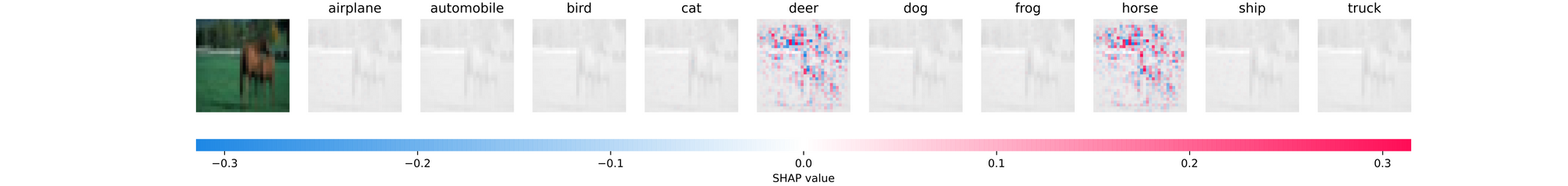
Form the output returned, the model correctly predicts this image instance as a Horse. The ensuing SHAP plot consists of the original image followed by 10 dim grayscale versions of itself. Each grayscale image is indicative of individual classes in the dataset and is labeled as such. Beneath the plot is a scale which reads from negative to positive, color coded from deep blue to bright red. This scale helps to show the intensity of the SHAP value assigned to each pertinent pixel.
Pixels colored deep blue are those which push the model away from predicting that the image belongs to that particular class while pixels colored bright red are those which strongly indicate that the image probably belongs to the class in question; white coloration on the other hand show that no importance was placed on those pixels by the model. Shades of colors in-between those mentioned vary proportionally.
Taking another look at the plot above it can be seen that the model has narrowed down it's gaze on two classes for that particular instance of data, Deer and Horse. In both classes, there are similar patterns of red pixels at the top of the image which implies that objects in that part of the image are synonymous to images of Deers and Horses (ie most Deers and Horses in the training set are pictured on a woodland background as seen in that data instance). However, looking at pixels along the position of the object of interest indicates that the Horse class possesses more red pixels in comparison to the Deer class. This means that the model has perceived that the shape of that object is more synonymous with that of a Horse.
Example 2

Consider the image instance above, again derived from the validation set. This image is correctly classified as a Deer but looking at the SHAP plots, one can see that the model had a more difficult time deciding which class the image belongs to when compared to the previous image. All of the classes are lit up with red and blue pixels in this case with classes automobile, bird and truck less lit than others.
The classes cat, deer, dog, frog and horse have the most activity on their grayscales, particularly on their backgrounds as it seems a significant number of the images in those classes contained in the training set are pictured on grass backgrounds. However, the model has classified the image as a Deer since there are less blue pixels overall compared to the other classes.
Example 3

Unlike the other two images, this data instance which is evidently a dog was misclassified as an airplane. On the surface this might seem like a rather bizarre classification but looking at the SHAP plots more light is shed on why the model behaved this way.
From the plot, both the airplane and the dog class were assumed to be most likely. However, unique differences are seen in the nature of SHAP values along the edges of the grayscales as the ear and neck region of the dog is mostly blue on airplane and red on dog, while regions along the outstretched feet of dog are lit red on airplane and blue on dog.
What this implies is that while the model recognizes that the head and neck region of the image is most likely that of a dog, the fact that the dog is in a stretched out position implies an aerodynamic shape which is most common in airplanes. It is most likely that there are not many images of dogs in that position in the training set for the model to properly learn that distinction.
Using Imported Images
By extending the function written in the previous section, we can make it so it receives an uploaded image, makes predictions and then provide model explainability via a SHAP plot. This is done below.
def plot_shap_util(filepath, mask, model):
  """
  This function performs model explainability
  by producing shap plots for a data instance
  """
  #  reading image and converting to tensor
  image = cv2.imread(filepath)
  image = cv2.cvtColor(image, cv2.COLOR_BGR2RGB)
  image = cv2.resize(image, (32, 32))
  image = transforms.ToTensor()(image)
  image = image.to(device)

  #-----------------
  #  CLASSIFICATION
  #-----------------
  #  creating a mapping of classes to labels
  label_dict = {0:'airplane', 1:'automobile', 2:'bird', 3:'cat', 4:'deer',
                5:'dog', 6:'frog', 7:'horse', 8:'ship', 9:'truck'}

  #  utilizing the model for classification
  prediction = torch.argmax(model(image), dim=1).item()

  #  displaying model classification
  print(f'prediction: {label_dict[prediction]}')

  #----------------
  #  EXPLANABILITY
  #----------------
  #  creating dataloader for mask
  mask_loader = DataLoader(mask, batch_size=200)

  #  creating explainer for model behaviour
  for images in mask_loader:
    images = images.to(device)
    explainer = shap.DeepExplainer(model, images)
    break

  #  deriving shap values for image of interest based on model behaviour
  shap_values = explainer.shap_values(image.view(-1, 3, 32, 32))

  #  preparing for visualization by changing channel arrangement
  shap_numpy = [np.swapaxes(np.swapaxes(x, 1, -1), 1, 2) for x in shap_values]
  test_numpy = np.swapaxes(np.swapaxes(image.view(-1, 3, 32, 32).cpu().numpy(), 1, -1), 1, 2)

  #  producing shap plots
  shap.image_plot(shap_numpy, test_numpy, show=False, labels= ['airplane', 'automobile', 'bird', 'cat', 'deer',
                                                               'dog', 'frog', 'horse', 'ship', 'truck'])

  pass
Using the extended function, we can then supply images as parameter and classification will be provided, followed by a SHAP plot which can then be interpreted for explainability.
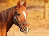
#  using the extended explainability function
plot_shap_util('image.jpg', mask, model.network)
In this case, the model has correctly classified the uploaded image as that of a Horse since it has less of blue pixels and more of red pixels compared to other classes. Though in this case, a localized region along the base of the image seem to play a huge role in this classification which is difficult to decipher.
Final Remarks
Model explainability helps to provide some useful insight into why a model behaves the way it does even though not all explanations may make sense or be easy to interpret. SHAP is just one way to explain outputs of deep learning models there exist numerous other libraries that can be used to the same effect.
Note: For this article, better explanations can be gotten with a better model. A better model in the context of better architecture and better model performance, feel free to change the model architecture or train the model for more epochs if deemed necessary.