Weather forecast using LSTM networks

Long Short-Term Memory (LSTM) networks are a class of recurrent neural network (RNN) that are capable of sequence prediction problems. RNNs and LSTMs in particular vary from other neural networks in that they have a temporal dimension and take time and sequence into account. In fact, they are considered to be the most effective and well-known subgroup of RNNs; they belong to a class of artificial neural networks made to identify patterns in data sequences, including numerical times series data. In this article, we will introduce

this subclass of networks and use it to build a Weather forecasting model.

What are Long Short Term Memory Networks ?

Long Short Term Memory (LSTM) networks are frequently used in sequence prediction problems. These recurrent neural networks have the capacity to learn sequence dependency. The output from the prior step is utilized as the upcoming step's input in the RNN. It was Hochreiter and Schmidhuber who originally created the Long-Short Term Memory architecture. It addressed the problem of "long-term reliance" in RNNs. This is where RNNs can predict variables based on information in the current data, but cannot predict variables held in long-term memory. However, the performance of RNN will not be improved by a growing gap length. By design, LSTMs are known to store data for a long time. This method is employed when analyzing time-series data, making predictions, and categorizing data.

Theoretically, classical RNNs are capable of tracking any kind of long-term dependencies in input sequences. However, plain RNNs have the drawback of not being applicable for real-world problems for this type of problems. The long-term gradients in back-propagated networks, for example, tend to decrease down to zero or increase up to infinity. This depends on the computations necessary for the process, which use a finite-precision number set.

Architecture of LSTM networks

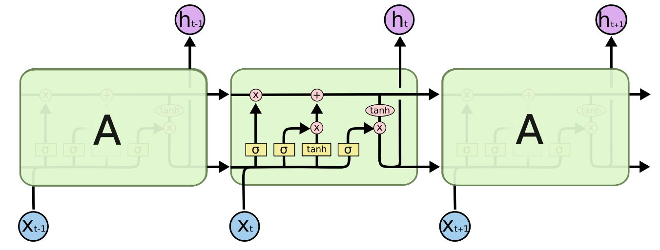
The architecture of LSTM networks uses four neural networks and multiple memory cells, or blocks, that create a chain structure make up the long-short term memory. A typical long-short term memory unit is made up of a cell, an input gate, an output gate, and a forget gate. The cell keeps track of values for any quantity of time, and the three gates regulate the flow of information into and out of the cell.

• Input gates: These gates select the input values that will be applied to modify the memory. These decide whether or not to pass through 0 or 1 data using the sigmoid function. Additionally, you may use the tanh function to give the data weights that represent their significance on a scale from -1 to 1.
• Forget gates: They are the gates responsible for the first step in the LSTM, which is to decide what information to throw away from the cell state. This decision is made based on a sigmoid layer. It looks at the previous state ht−1 and the input xt, and generates a number between 0 and 1 for each value in the cell state Ct−1. A 1 represents a completely preserved value while a 0 represents a completely forgotten one.
• Output gates: This final class of gates determines what data will be send to the output. This output, however filtered, will be based on the state of our cell. We first run a sigmoid layer to determine which portions of the cell state will be output. Then, in order to output only the portions we decided to, we multiply the cell state by the output of the sigmoid gate after passing the cell state through tanh to force the values to fall in the range of -1 and 1.

Weather Data set

Due to the constant need for weather forecast and disaster prediction. Weather datasets are one of the most present and accessible online. In this tutorial, we will use the Jena Climate dataset recorded by the Max Planck Institute for Biogeochemistry.

This is a time series dataset for the city of Jena in Germany with records spanning 10 minutes and consisting of 14 features (temperature, relative humidity, pressure...). It is available for different date ranges, but we will be using the 6 month record for the second semester of 2021 at the university.

Let's start by downloading the dataset to our Gradient Notebook:

!curl https://www.bgc-jena.mpg.de/wetter/mpi_saale_2021b.zip -o mpi_saale_2021b.zip

Then, we will extract the zip contents into a csv file, and link the content of this one to a data frame with the library pandas.

import zipfile
import pandas

zip_file = zipfile.ZipFile("mpi_saale_2021b.zip")
zip_file.extractall()
csv_path = "mpi_saale_2021b.csv"
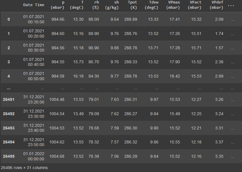
data_frame = pandas.read_csv(csv_path)

This data frame will contain the 26495 rows of the 6 month timestamp records of the aforementioned 14 weather features of the Jena region.

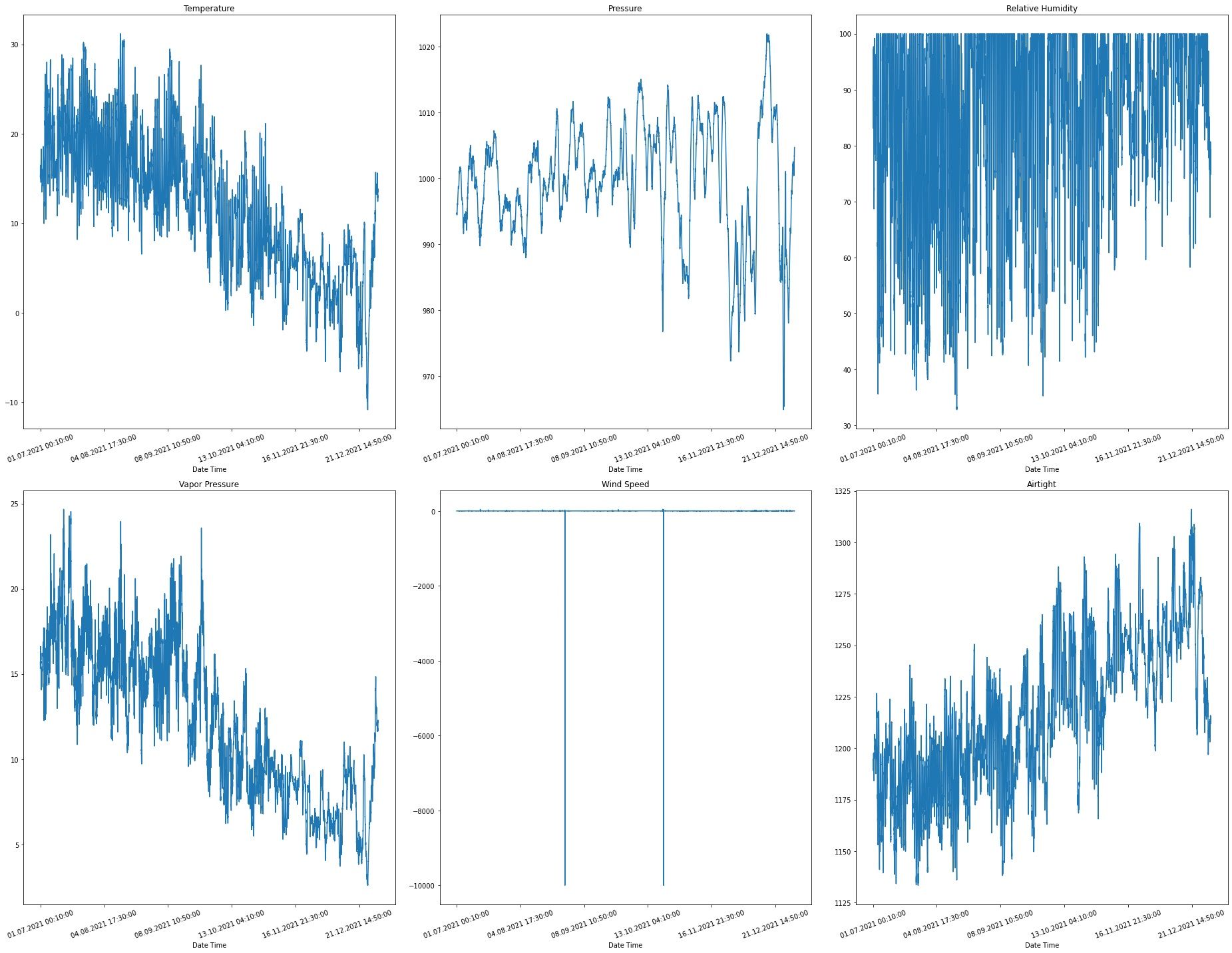
For long time prediction (up to 1 or 2 months), the full spectrum of features should be taken into consideration. In our case, for demonstration purposes of the LSTM network we will be forecasting the weather for different periods ranging from a few hours up to a few days. So, we will be using, beside the time, only six features: temperature, pressure, relative humidity, vapor pressure, wind speed and airtight.

time = data_frame['Date Time']
temperature = data_frame['T (degC)']
pressure = data_frame['p (mbar)']
relative_humidity = data_frame['rh (%)']
vapor_pressure = data_frame['VPact (mbar)']
wind_speed = data_frame['wv (m/s)']
airtight = data_frame['rho (g/m**3)']

Using Matplotlib, we can show the graph over time of these features

import matplotlib.pyplot as plt
from matplotlib.pyplot import figure

plt.subplots(nrows=2, ncols=3, figsize=(26, 20))

ax = plt.subplot(2, 3, 1)
temperature.index = time
temperature.head()
temperature.plot(rot=20)
plt.title('Temperature')

ax = plt.subplot(2, 3, 2)
pressure.index = time
pressure.head()
pressure.plot(rot=20)
plt.title('Pressure')

ax = plt.subplot(2, 3, 3)
relative_humidity.index = time
relative_humidity.head()
relative_humidity.plot(rot=20)
plt.title('Relative Humidity')

ax = plt.subplot(2, 3, 4)
vapor_pressure.index = time
vapor_pressure.head()
vapor_pressure.plot(rot=20)
plt.title('Vapor Pressure')

ax = plt.subplot(2, 3, 5)
wind_speed.index = time
wind_speed.head()
wind_speed.plot(rot=20)
plt.title('Wind Speed')

ax = plt.subplot(2, 3, 6)
airtight.index = time
airtight.head()
airtight.plot(rot=20)
plt.title('Airtight')

plt.tight_layout()
plt.show()

 This will result in the following image:

Data Preprocessing

Down-sampling

We are choosing 26,000 data points in this case for training. A recording of an observation is made every 10 minutes, or six times an hour. Since no significant change is anticipated over 60 minutes, we will resample the data set down to a single record every hour. This can be executed via the parameter sampling_rate of the method timeseries_dataset_from_array from Keras preprocessing library. So, this argument should be set to 6 to have the required down-sample we are looking for.

Data normalization

Before training the neural network, we perform normalization to limit feature values to a range from 0 to 1 because each feature has values with variable ranges. To accomplish this, we divide each feature's standard deviation by its mean before deducting it.

def normalize(data):
    data_mean = data.mean(axis=0)
    data_std = data.std(axis=0)
    return (data - data_mean) / data_std

So, let's group the selected features into a single array to apply this normalization function

features = pandas.concat([temperature, pressure, relative_humidity, vapor_pressure, wind_speed, airtight], axis=1)
features.index = time
features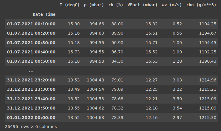

features = normalize(features.values)
features = pandas.DataFrame(features)
features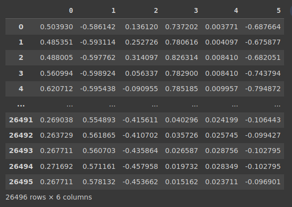

Then, we will split the dataset into training and validation by allocation 80% of the dataset to the training

training_size = int ( 0.8 * features.shape[0])  
train_data = features.loc[0 : training_size - 1]
val_data = features.loc[training_size:]

Training dataset

For each prediction, we will be using the tracking data from the past 3 days, which is equivalent to around 432 timestamp ( 3 × 24 × 6 = 432 ).
This data will be used to predict the temperature after 6 hours into the future, which is equivalent to 36 timestamps before down-sampling.

start = 432 + 36
end = start + training_size

x_train = train_data.values
y_train = features.iloc[start:end][[0]]

sequence_length = int(432 / 6)

Then let's construct the training dataset in its final form using the Keras preprocessing library

from tensorflow import keras

dataset_train = keras.preprocessing.timeseries_dataset_from_array(
    data=x_train,
    targets=y_train,
    sequence_length=sequence_length,
    sampling_rate=6,
    batch_size=64,
)

Validation dataset

In a similar way, we will construct the validation set. However, the last 468 (432 + 36) rows must be excluded from the data because we won't have label information for those entries. Let's take the 468 rows away from the end of the data. Also, the validation label dataset must begin at position 468 after the training split position.

x_val_end = len(val_data) - start

label_start = training_size + start

x_val = val_data.iloc[:x_val_end][[i for i in range(6)]].values
y_val = features.iloc[label_start:][[0]]

dataset_val = keras.preprocessing.timeseries_dataset_from_array(
    x_val,
    y_val,
    sequence_length=sequence_length,
    sampling_rate=6,
    batch_size=64,
)

Creating an LSTM Weather Forecast Model

First, let's extract a single batch from the training dataset and use it to have the input and output layer dimension. Then, we will use the Keras layers library to create an LSTM layer with 32 memory units.

for batch in dataset_train.take(1):
    inputs, targets = batch
    
inputs = keras.layers.Input(shape=(inputs.shape[1], inputs.shape[2]))
lstm_out = keras.layers.LSTM(32)(inputs)
outputs = keras.layers.Dense(1)(lstm_out)

model = keras.Model(name="Weather_forcaster",inputs=inputs, outputs=outputs)
model.compile(optimizer=keras.optimizers.Adam(learning_rate=0.001), loss="mse")
model.summary()

The summary of this model is as follows

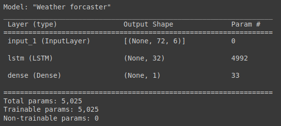
Then, we fit the model using the training/validation datasets and an epoch number of 15 (determined experimentally for our dataset).

history = model.fit(
    dataset_train,
    epochs=15,
    validation_data=dataset_val
)

Next, we show the results of fitting the model in terms of training loss below.

loss = history.history["loss"]
epochs = range(len(loss))
plt.figure()
plt.plot(epochs, loss, "b", label="Training loss")
plt.title("Training Loss")
plt.xlabel("Epochs")
plt.ylabel("Loss")
plt.show()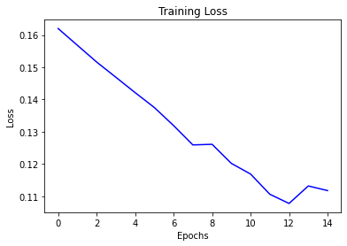

After getting our trained model, we will use it to predict the normalized temperature for a value in the validation dataset. Then, we will denormalize this value using the standard deviation and mean of the temperature, and plot the results in a plot using Matplotlib.

temp_mean = temperature.mean(axis=0)
temp_std = temperature.std(axis=0)

for x, y in dataset_val.skip(12):
    history_data = x[0][:, 1].numpy() * temp_std + temp_mean
    true_value = y[0].numpy() * temp_std + temp_mean
    prediction = model.predict(x)[0] * temp_std + temp_mean
    time_steps = list(range(-(history_data.shape[0]), 0))
    plt.plot(time_steps, history_data)
    plt.plot(36, true_value, "gD")
    plt.plot(36, prediction, "rX")
    plt.legend(["History", "True Future", "Model Prediction"])
    plt.xlabel("Time")
    plt.show()
    break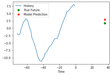

Conclusion

Long Short-Term Memory networks are a type of recurrent neural network that may solve problems involving sequence prediction. RNNs and LSTMs, in particular, differ from other neural networks in that they contain a temporal dimension and account for time and sequence. In this post, we presented this network subclass and used it to construct a weather forecasting model. We proved its effectiveness as a subgroup of RNNs designed to detect patterns in data sequences, including numerical time series data.

Resources

http://www.bioinf.jku.at/publications/older/2604.pdf

https://www.researchgate.net/publication/13853244_Long_Short-term_Memory

https://www.bgc-jena.mpg.de/wetter/

https://keras.io/api/layers/recurrent_layers/lstm/

https://keras.io/examples/timeseries/timeseries_weather_forecasting/