Bring this project to life
Convolutional neural networks take in a 2-dimensional spatial structured data instance (an image), and process it until a 1-dimensional vector representation of some sort is produced. It the begs the question, if a mapping can be learnt from an image matrix to a vector representation, perhaps a mapping can be learnt from that vector representation back to an image. In this demo article, we will be exploring just that.
Convnets as Feature Extractors
In previous articles, I had touched on the fact that convolution layers in a convnet serve the purpose of extracting features from images. Those features are then passed unto linear layers which perform the actual classification (exceptions are made for architectures that utilize 1 x 1 convolution layers for downsampling).
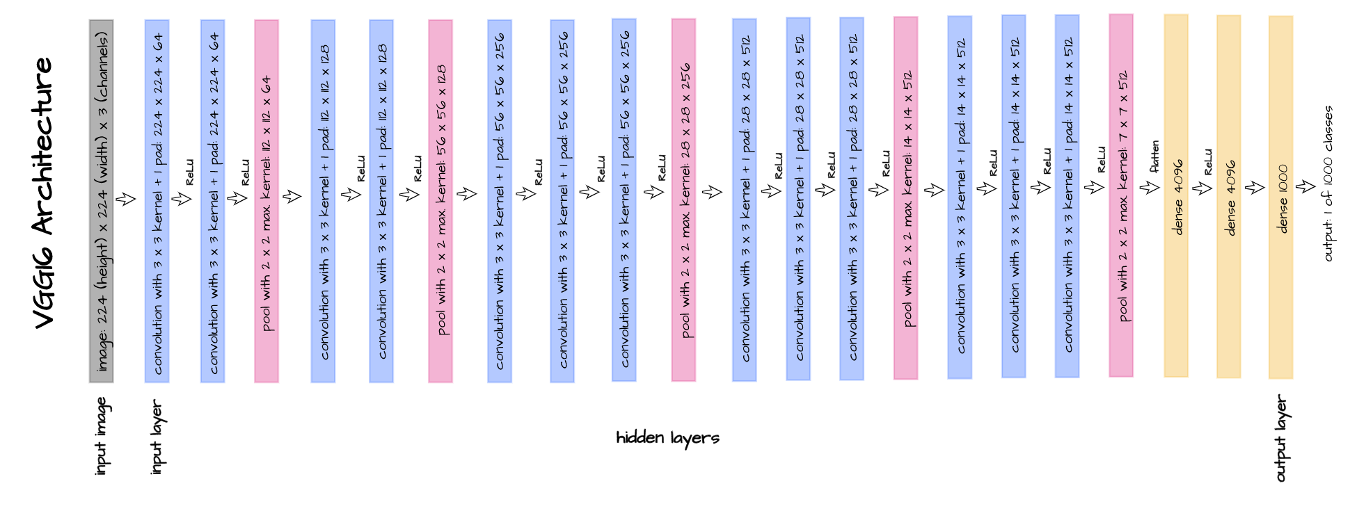
Consider VGG-16 with it's architecture depicted above, from the input layer right till the point where the pooled 7 x 7 x 512 feature maps are flattened to create a vector of size 25,088 elements: that portion of the network serves as a feature extractor. Essentially, a 224 x 224 image with a total of 50,176 pixels is processed to create a 25,088 element feature vector, and this feature vector is then passed to the linear layers for classification.
Since these features are extracted by a convnet, it is logical to assume that another convnet could possibly make sense of these features, and put the original image that those features belong to back together, basically reversing the feature extraction process. This is essentially what an Autoencoder does.
Structure of an Autoencoder
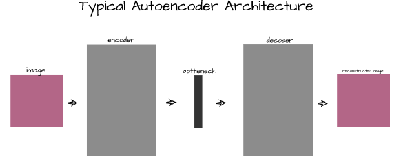
As stated in the previous section, autoencoders are deep learning architectures capable of reconstructing data instances from their feature vectors. They work on all sorts of data but this article is primarily concerned with their application on image data. An autoencoder is made up of 3 main components; namely, an encoder, a bottleneck and a decoder.
Encoder
The first section of an autoencoder, the encoder is the convnet that acts specifically as a feature extractor. Its primary function is to help extract the most salient features from images and return them as a vector.
Bottleneck
Located right after the encoder, the bottleneck, also called a code layer, serves as an extra layer which helps to compress the extracted features into a smaller vector representation. This is done in a bid to make it more difficult for the decoder to make sense of the features and force it to learn more complex mappings.
Decoder
The last section of an autoencoder, the decoder is that convnet which attempts to make sense of the features coming from the encoder, which have been subsequently compressed in the bottleneck, so as to reconstruct the original image as it was.
Training an Autoencoder
In this section we shall be implementing an autoencoder from scratch in PyTorch and training it on a specific dataset.
Let's start by quickly importing our required packages.
#  article dependencies
import torch
import torch.nn as nn
import torch.nn.functional as F
import torchvision
import torchvision.transforms as transforms
import torchvision.datasets as Datasets
from torch.utils.data import Dataset, DataLoader
import numpy as np
import matplotlib.pyplot as plt
import cv2
from tqdm.notebook import tqdm
from tqdm import tqdm as tqdm_regular
import seaborn as sns
from torchvision.utils import make_grid
import random
# configuring device
if torch.cuda.is_available():
device = torch.device('cuda:0')
print('Running on the GPU')
else:
device = torch.device('cpu')
print('Running on the CPU')Preparing Data
For the purpose of this article, we will utilize the CIFAR-10 dataset in training a convolutional autoencoder. It can be loaded as seen in the code cell below.
#  loading training data
training_set = Datasets.CIFAR10(root='./', download=True,
                              transform=transforms.ToTensor())

#  loading validation data
validation_set = Datasets.CIFAR10(root='./', download=True, train=False,
                                transform=transforms.ToTensor())
Next we need to extract only the images from the dataset. Since we are trying to teach an autoencoder to reconstruct images, the targets will not be class labels but the actual images themselves. An image from each class is also extracted and stored in the object 'test_images' just for visualization purposes, more on this later.
def extract_each_class(dataset):
  """
  This function searches for and returns
  one image per class
  """
  images = []
  ITERATE = True
  i = 0
  j = 0

  while ITERATE:
    for label in tqdm_regular(dataset.targets):
      if label==j:
        images.append(dataset.data[i])
        print(f'class {j} found')
        i+=1
        j+=1
        if j==10:
          ITERATE = False
      else:
        i+=1

  return images


#  extracting training images
training_images = [x for x in training_set.data]

#  extracting validation images
validation_images = [x for x in validation_set.data]

#  extracting test images for visualization purposes
test_images = extract_each_class(validation_set)
Now we need to define a PyTorch dataset class so as to be able to use the images as tensors. This along with class instantiation is done in the code cell below.
#  defining dataset class
class CustomCIFAR10(Dataset):
  def __init__(self, data, transforms=None):
    self.data = data
    self.transforms = transforms

  def __len__(self):
    return len(self.data)

  def __getitem__(self, idx):
    image = self.data[idx]

    if self.transforms!=None:
      image = self.transforms(image)
    return image


#  creating pytorch datasets
training_data = CustomCIFAR10(training_images, transforms=transforms.Compose([transforms.ToTensor(),
                                                                              transforms.Normalize((0.5, 0.5, 0.5), (0.5, 0.5, 0.5))]))
validation_data = CustomCIFAR10(validation_images, transforms=transforms.Compose([transforms.ToTensor(),
                                                                                  transforms.Normalize((0.5, 0.5, 0.5), (0.5, 0.5, 0.5))]))
test_data = CustomCIFAR10(test_images, transforms=transforms.Compose([transforms.ToTensor(),
                                                                                  transforms.Normalize((0.5, 0.5, 0.5), (0.5, 0.5, 0.5))]))
Autoencoder Architecture
A custom convolutional autoencoder architecture is defined for the purpose of this article as illustrated below. This architecture is designed to work with the CIFAR-10 dataset as its encoder takes in 32 x 32 pixel images with 3 channels and processes them until 64 8 x 8 feature maps are produced.
These feature maps are then flattened to produce a vector of 4096 elements which is then compressed to just 200 elements in the bottleneck. The decoder takes this 200 element vector representation and processes it via transposed convolution until a 3 x 32 x 32 image is returned as output.
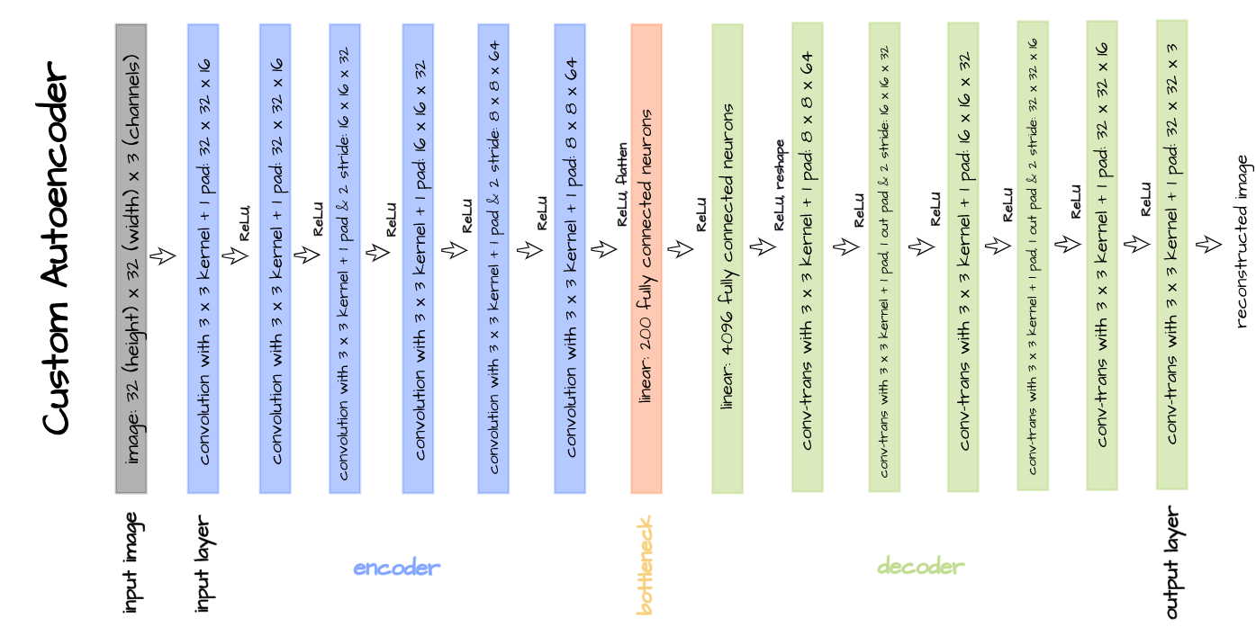
The above defined architecture is implemented in the code cell below. The parameter 'latent_dim' in this instance refers to the size of the bottleneck which we have specified to be 200.
#  defining encoder
class Encoder(nn.Module):
  def __init__(self, in_channels=3, out_channels=16, latent_dim=200, act_fn=nn.ReLU()):
    super().__init__()

    self.net = nn.Sequential(
        nn.Conv2d(in_channels, out_channels, 3, padding=1), # (32, 32)
        act_fn,
        nn.Conv2d(out_channels, out_channels, 3, padding=1),
        act_fn,
        nn.Conv2d(out_channels, 2*out_channels, 3, padding=1, stride=2), # (16, 16)
        act_fn,
        nn.Conv2d(2*out_channels, 2*out_channels, 3, padding=1),
        act_fn,
        nn.Conv2d(2*out_channels, 4*out_channels, 3, padding=1, stride=2), # (8, 8)
        act_fn,
        nn.Conv2d(4*out_channels, 4*out_channels, 3, padding=1),
        act_fn,
        nn.Flatten(),
        nn.Linear(4*out_channels*8*8, latent_dim),
        act_fn
    )

  def forward(self, x):
    x = x.view(-1, 3, 32, 32)
    output = self.net(x)
    return output


#  defining decoder
class Decoder(nn.Module):
  def __init__(self, in_channels=3, out_channels=16, latent_dim=200, act_fn=nn.ReLU()):
    super().__init__()

    self.out_channels = out_channels

    self.linear = nn.Sequential(
        nn.Linear(latent_dim, 4*out_channels*8*8),
        act_fn
    )

    self.conv = nn.Sequential(
        nn.ConvTranspose2d(4*out_channels, 4*out_channels, 3, padding=1), # (8, 8)
        act_fn,
        nn.ConvTranspose2d(4*out_channels, 2*out_channels, 3, padding=1,
                           stride=2, output_padding=1), # (16, 16)
        act_fn,
        nn.ConvTranspose2d(2*out_channels, 2*out_channels, 3, padding=1),
        act_fn,
        nn.ConvTranspose2d(2*out_channels, out_channels, 3, padding=1,
                           stride=2, output_padding=1), # (32, 32)
        act_fn,
        nn.ConvTranspose2d(out_channels, out_channels, 3, padding=1),
        act_fn,
        nn.ConvTranspose2d(out_channels, in_channels, 3, padding=1)
    )

  def forward(self, x):
    output = self.linear(x)
    output = output.view(-1, 4*self.out_channels, 8, 8)
    output = self.conv(output)
    return output


#  defining autoencoder
class Autoencoder(nn.Module):
  def __init__(self, encoder, decoder):
    super().__init__()
    self.encoder = encoder
    self.encoder.to(device)

    self.decoder = decoder
    self.decoder.to(device)

  def forward(self, x):
    encoded = self.encoder(x)
    decoded = self.decoder(encoded)
    return decoded
Per usual, we now need to define a class which will help make training and validation more seamless. In this case, since we are training a generative model, losses might not carry too much information. In general, we want loss to be reduced, and we also can use loss values to be able to see how well the autoencoder reconstructs images for every epoch. For this reason, I have included a visualization block as seen below.
class ConvolutionalAutoencoder():
  def __init__(self, autoencoder):
    self.network = autoencoder
    self.optimizer = torch.optim.Adam(self.network.parameters(), lr=1e-3)

  def train(self, loss_function, epochs, batch_size,
            training_set, validation_set, test_set):

    #  creating log
    log_dict = {
        'training_loss_per_batch': [],
        'validation_loss_per_batch': [],
        'visualizations': []
    }

    #  defining weight initialization function
    def init_weights(module):
      if isinstance(module, nn.Conv2d):
        torch.nn.init.xavier_uniform_(module.weight)
        module.bias.data.fill_(0.01)
      elif isinstance(module, nn.Linear):
        torch.nn.init.xavier_uniform_(module.weight)
        module.bias.data.fill_(0.01)

    #  initializing network weights
    self.network.apply(init_weights)

    #  creating dataloaders
    train_loader = DataLoader(training_set, batch_size)
    val_loader = DataLoader(validation_set, batch_size)
    test_loader = DataLoader(test_set, 10)

    #  setting convnet to training mode
    self.network.train()
    self.network.to(device)

    for epoch in range(epochs):
      print(f'Epoch {epoch+1}/{epochs}')
      train_losses = []

      #------------
      #  TRAINING
      #------------
      print('training...')
      for images in tqdm(train_loader):
        #  zeroing gradients
        self.optimizer.zero_grad()
        #  sending images to device
        images = images.to(device)
        #  reconstructing images
        output = self.network(images)
        #  computing loss
        loss = loss_function(output, images.view(-1, 3, 32, 32))
        #  calculating gradients
        loss.backward()
        #  optimizing weights
        self.optimizer.step()

        #--------------
        # LOGGING
        #--------------
        log_dict['training_loss_per_batch'].append(loss.item())

      #--------------
      # VALIDATION
      #--------------
      print('validating...')
      for val_images in tqdm(val_loader):
        with torch.no_grad():
          #  sending validation images to device
          val_images = val_images.to(device)
          #  reconstructing images
          output = self.network(val_images)
          #  computing validation loss
          val_loss = loss_function(output, val_images.view(-1, 3, 32, 32))

        #--------------
        # LOGGING
        #--------------
        log_dict['validation_loss_per_batch'].append(val_loss.item())


      #--------------
      # VISUALISATION
      #--------------
      print(f'training_loss: {round(loss.item(), 4)} validation_loss: {round(val_loss.item(), 4)}')

      for test_images in test_loader:
        #  sending test images to device
        test_images = test_images.to(device)
        with torch.no_grad():
          #  reconstructing test images
          reconstructed_imgs = self.network(test_images)
        #  sending reconstructed and images to cpu to allow for visualization
        reconstructed_imgs = reconstructed_imgs.cpu()
        test_images = test_images.cpu()

        #  visualisation
        imgs = torch.stack([test_images.view(-1, 3, 32, 32), reconstructed_imgs],
                          dim=1).flatten(0,1)
        grid = make_grid(imgs, nrow=10, normalize=True, padding=1)
        grid = grid.permute(1, 2, 0)
        plt.figure(dpi=170)
        plt.title('Original/Reconstructed')
        plt.imshow(grid)
        log_dict['visualizations'].append(grid)
        plt.axis('off')
        plt.show()

    return log_dict

  def autoencode(self, x):
    return self.network(x)

  def encode(self, x):
    encoder = self.network.encoder
    return encoder(x)

  def decode(self, x):
    decoder = self.network.decoder
    return decoder(x)
With everything set, we can then instantiate our autoencoder as a member of the convolutional autoencoder class we defined below using the parameters as specified in the code cell that follows.
Bring this project to life
# training model
model = ConvolutionalAutoencoder(Autoencoder(Encoder(), Decoder()))
log_dict = model.train(nn.MSELoss(), epochs=10, batch_size=64,
training_set=training_data, validation_set=validation_data,
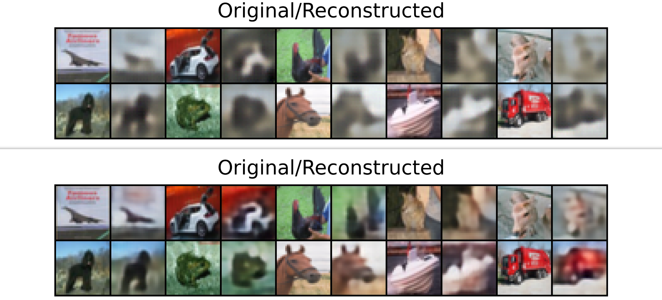
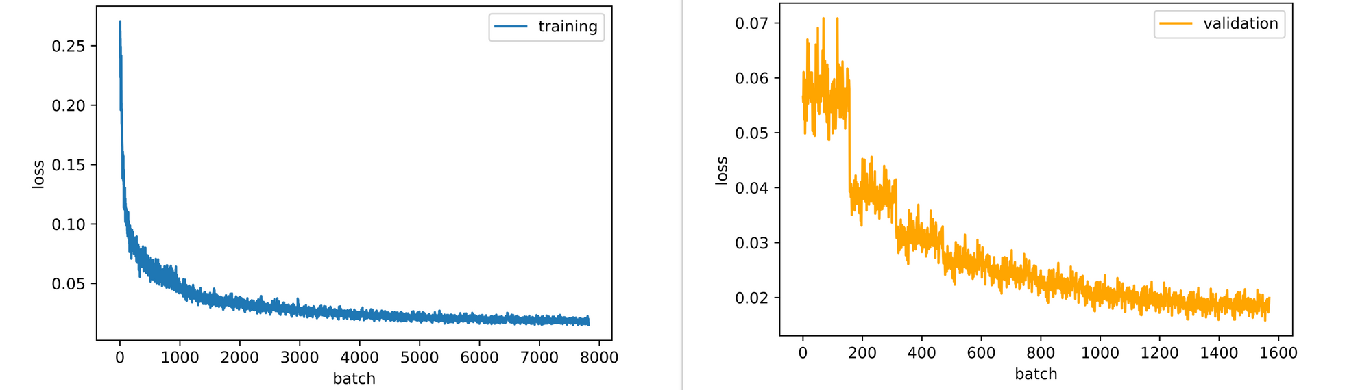
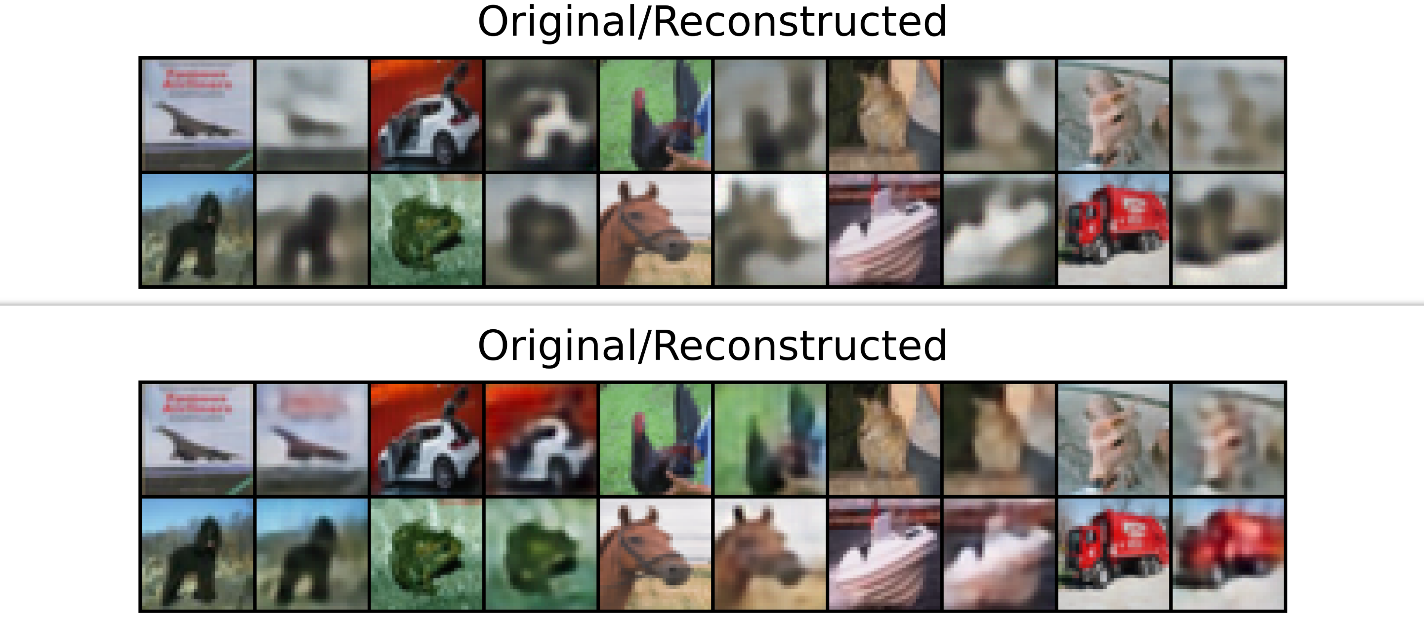
test_set=test_data)Right from the end of the first epoch, it is evident that our decoder has begun to develop a sense of how to reconstruct images fed into the encoder, even though it only had access to a compressed 200 element feature vector representation. Reconstructed images continue to increase in detail right up till the 10th epoch as well.
Looking at the training and validation losses, the autoencoder could still benefit slightly from some more epochs of training as it's losses are still down-trending. This is the case for the validation loss more so than training loss, which seems to be plateauing.
Bottleneck and Details
In one of the previous sections, I had mentioned how the bottleneck code layer serves the purpose of further compressing a feature vector, so as to force the decoder to learn a more complex and generalizable mapping. On the flip side, a fine balance is to be sought as the magnitude of compression in the code layer would also influence how well a decoder can reconstruct an image.
The smaller the vector representation passed to the decoder, the less image features the decoder has access to and the less detailed its reconstructions will be. In the same sense, the bigger the the vector representation passed to the decoder, the more image features it has access to and the more detailed its reconstructions will be. Following this line of thinking, let's train the same autoencoder architecture, but this time using a bottleneck of size 1000.
# training model
model = ConvolutionalAutoencoder(Autoencoder(Encoder(latent_dim=1000), Decoder(latent_dim=1000)))
log_dict = model.train(nn.MSELoss(), epochs=10, batch_size=64,
training_set=training_data, validation_set=validation_data,
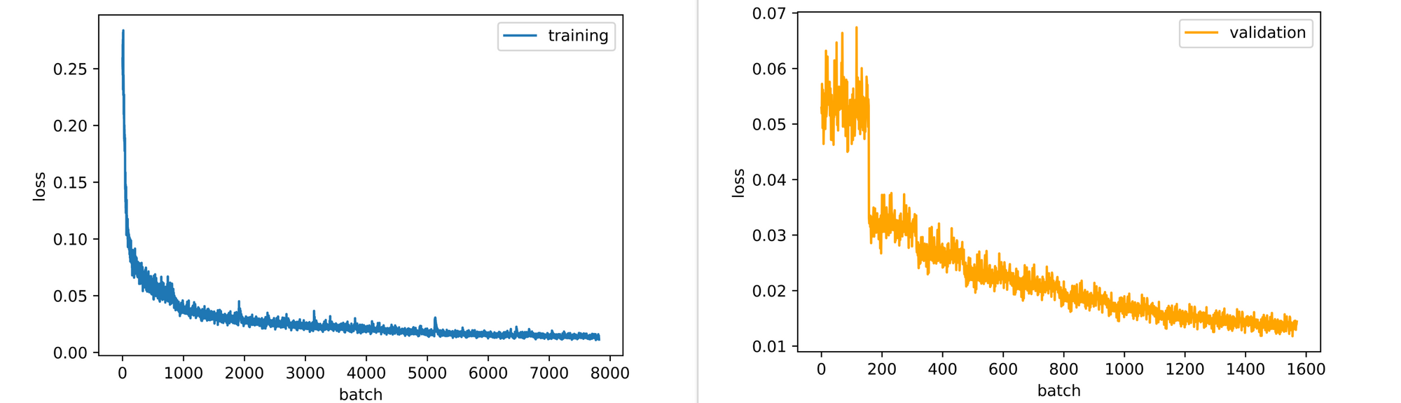
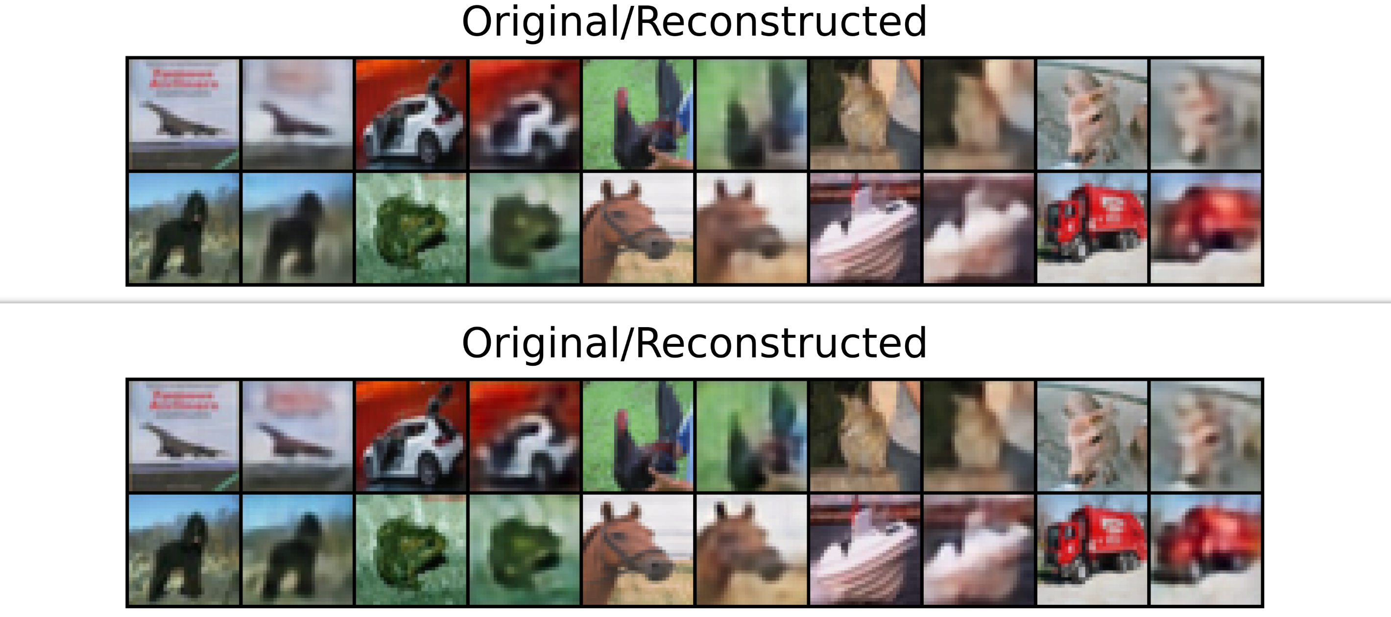
test_set=test_data)From the visualizations generated per epoch, it is immediately evident that the decoder does a better job at reconstructing images in terms of detail and visual accuracy. This goes down to the fact that the new decoder has access to more features, as the original feature vector of 4096 elements is now downsampled to 1000 elements instead of 200.
Again, the autoencoder could benefit from some more epochs of training. It's training and validation losses are still down-trending, with slopes steeper than those we observed when we trained our autoencoder with a bottleneck of just 200 elements.
Comparing bottlenecks of size 200 and 1000 both at the 10th epoch shows clearly that images generated with a bottleneck of 1000 elements are clearer/more detailed than those generated with a bottleneck of 200 elements.
Training to Absolute Refinement
At what point is a convolutional autoencoder optimally trained? From the two autoencoders we have trained we can observe that reconstructions are still blurry at the 10th epoch even though our loss plots had began to flatten. Increasing the bottleneck size will only ameliorate this issue to an extent, but will not completely solve it.
This is partly down to the loss function used in this case, mean squared error, as it does not do too well while measuring losses in generative models. For the most part, these blurry reconstructions are the bane of convolutional autoencoders tasks. If one's goal is to reconstruct or generate images, a generative adversarial network (GAN) or diffusion model may be a safer bet. However, that is not to say that convolutional autoencoders are not useful as they can be used for anomaly detection, image denoising and so on.
Final Remarks
In this article, we discussed autoencoders in the context of image data. We went on to take a look at what exactly a convolutional autoencoder does, and how it does it with a view at developing an intuition of it's working principle. Thereafter, we touched on its different section before going further to define a custom autoencoder of our own, training it and discussing the results of the model training.