Over the years, we have seen very powerful models being built to distinguish between objects. These models keep getting better in terms of performance and latency day by day but have we ever wondered what exactly these models pick up from images used to train them to make practically flawless predictions. There are undoubtedly features in images we feed into these models that they look at to make predictions and that is what we seek to explore in this article. Not long ago, researchers at Stanford university released a paper https://arxiv.org/abs/1901.07031 on how they are using deep learning to push the edge of Pneumonia diagnosis. Their work really got me fascinated so I tried it out in Pytorch and I am going to show you how I implemented this work using a different dataset on Kaggle.
Link to paper on Class Activation Maps: http://cnnlocalization.csail.mit.edu/Zhou_Learning_Deep_Features_CVPR_2016_paper.pdf
In this post, we’ll build a machine learning pipeline to classify whether a patient has Pneumonia or not from chest x-ray images and then draw a heat-map on areas that the model used to make these decisions. Below is a quick overview of the entire project.
Load and preprocess our data

Feed the data into the model and train
Perform both forward pass and backward pass to train our model
Test and evaluate our model
Model evaluation

And then lastly we draw class activation maps on our test samples to generate our final desired output
Pneumonia sample

LOGIC
Our goal in this project is to classify chest x-ray images as containing Pneumonia or not and draw class activation maps on discriminative regions used to identify the Pneumonia. We are going to leverage the simple nature of the connectivity offered by Global Average Pooling in already existing canonical models to design a pipeline to perform the task at hand. Since ResNet already has a Global Average Pooling, we find it ideal for use for this task.In order to get a full grasp of the task at hand, there are some areas in the model we will want to visit. One important area is the Global Average Pooling layer.
GLOBAL AVERAGE POOLING LAYER
Usually in a Convolutional Neural Network architecture, all the convolutional layers are proceeded by one or more fully connected layers but these fully connected layers normally have a lot of parameters making the model prone to over-fitting. The Global Average Pooling layer as a replacement to fully connected layers at the end of convolutional layers reduces the number of parameters due to the fully connected layers to zero since they just reduce the spatial dimension to feature maps produced by the last convolutional layer. They work exactly the same way as average and max pooling layers but perform a more extreme dimensional reduction by taking a tensor of size h x w x d and producing a tensor of size 1 x 1 x d. All what they do is to find the average each h x w feature map into a singe value.

DATASET
For this project, we are going to use a dataset available at kaggle consisting of 5433 training datapoints, 624 validation datapoints and 16 test datapoints.
Link to dataset: https://www.kaggle.com/paultimothymooney/chest-xray-pneumonia
MODEL ARCHITECTURE
Our base line model for this project is the ResNet 152. ResNet models like other convolutional network architectures consist of series of convolutional layers but designed in a way to favor very deep networks. The convolutional layers are arranged in series of Residual blocks. The significance of these Residual blocks is to prevent the problem of vanishing gradients which are very pervasive in very deep convolutional networks. Residual blocks have skip connections which allow gradient flow in very deep networks.

BUILDING AND TRAINING OUR MODEL FOR CLASSIFICATION.
Let's remind ourselves that our main goal is to draw heap-maps on discriminative regions used to identify Pneumonia in chest x-ray images but in order to achieve that goal, we must train our model to perform normal classification. We are going to build our model in an object oriented programming style, a conventional way to build models in Pytorch. First thing to do in building our model is to import all the required packages. The packages required for this project are as follows:
- Torch (torch.nn, torch.optim, torchvision, torchvision.transforms)
- Numpy
- Matplotlib
- Scipy
- PIL
Pytorch provides us with incredibly powerful libraries to load and preprocess our data without writing any boilerplate code. We will use the Dataset module and the ImageFolder module to load our data from the directory containing the images and apply some data augmentation to generate different variants of the images.
#Using the transforms module in the torchvision module, we define a set of functions that perform data augmentation on our dataset to obtain more data.#
transformers = {'train_transforms' : transforms.Compose([
    transforms.Resize((224,224)),
    #transforms.CenterCrop(224),
    transforms.RandomRotation(20),
    transforms.RandomHorizontalFlip(),
    transforms.ToTensor(),
    transforms.Normalize([0.485, 0.456, 0.406], std=[0.229, 0.224, 0.225])
]),
'test_transforms' : transforms.Compose([
    transforms.Resize((224,224)),
    transforms.CenterCrop(224),
    transforms.ToTensor(),
    transforms.Normalize([0.485, 0.456, 0.406], std=[0.229, 0.224, 0.225])
]),
'valid_transforms' : transforms.Compose([
    transforms.Resize((224,224)),
    transforms.CenterCrop(224),
    transforms.ToTensor(),
    transforms.Normalize([0.485, 0.456, 0.406], std=[0.229, 0.224, 0.225])
])}
trans = ['train_transforms','valid_transforms','test_transforms']
path = "/content/gdrive/My Drive/chest_xray/"
categories = ['train','val','test']
Using the torchvision.datasets.ImageFolder module we load images from our dataset directory.
dset = {x : torchvision.datasets.ImageFolder(path+x, transform=transformers[y]) for x,y in zip(categories, trans)}
dataset_sizes = {x : len(dset[x]) for x in ["train","test"]}
num_threads = 4

#By passing a dataset instance into a DataLoader module, we create dataloader which generates images in batches.
dataloaders =  {x : torch.utils.data.DataLoader(dset[x], batch_size=256, shuffle=True, num_workers=num_threads)
               for x in categories}
Now that we are done loading our datasets, we can go ahead and take a look at some samples using the snippet below.
def imshow(inp, title=None):
    inp = inp.numpy().transpose((1,2,0))
    mean = np.array([0.485, 0.456, 0.406])
    std = np.array([0.229, 0.224, 0.225])
    inp = std*inp + mean
    inp = np.clip(inp,0,1)
    plt.imshow(inp)
    if title is not None:
        plt.title(title)
    plt.pause(0.001)
inputs,classes = next(iter(dataloaders["train"]))
out = torchvision.utils.make_grid(inputs)
class_names = dataset["train"].classes
imshow(out, title = [class_names[x] for x in classes])
Samples Generated. Please take note that you should reduce your batch size to produce larger samples to view.
We have just verified that our data is being loaded correctly so we can move on to build our model.As I mentioned earlier, we are going to build our model in an object oriented programming style. Our model class is going to inherit from the nn.Module provided by PyTorch. The nn.Module just like in other machine learning frameworks like TensorFlow provides us with all the functionality we need to build a neural network. You can visit https://pytorch.org/docs/stable/_modules/torch/nn/modules/module.html for more info.
After defining our model class and inheriting from the nn.Module, we define the graph of our model in the init constructor by leveraging the feature extractor of ResNet-152 through a technique called transfer learning. The torchvision module provides us with state of the art models that have been trained on very huge datasets(ImageNet) and hence have very powerful feature extractors. Pytorch provides us with the ability to take and freeze these powerful feature extractors, attach our own classifiers depending on our problem domain and train the resulting model to suit our problem.
class Model(nn.Module):
    def __init__(self):
        super(Model, self).__init__()
        #obtain the ResNet model from torchvision.model library
        self.model = torchvision.models.resnet152(pretrained=True)
        #build our classifier and since we are classifying the images into NORMAL and PNEMONIA, we output a two-dimensional tensor.
        self.classifier = nn.Sequential(
        nn.Linear(self.model.fc.in_features,2),
        nn.LogSoftmax(dim=1))
        #Requires_grad = False denies the ResNet model the ability to update its parameters hence make it unable to train.
        for params in self.model.parameters():
            params.requires_grad = False
            #We replace the fully connected layers of the base model(ResNet model) which served as the classifier with our custom trainable classifier.
        self.model.fc = self.classifier
Every model built from the nn.Module requires that we override the forward function we defines the forward pass computation performed at every call.
def forward(self, x):
    # x is our input data
    return self.model(x)
Before you proceed to the part below, I recommend taking this 60 minute blitz tutorial on the Pytorch official page: https://pytorch.org/tutorials/beginner/deep_learning_60min_blitz.html but if you still opt to proceed, don’t worry, I will do my very best to explain every bit of the code in the comments in the code.Next part of our training process is to define a fit function(Not obligatory to define in the model class) where we basically train our model on the dataset. Let’s look at the code to do so.
def fit(self, dataloaders, num_epochs):
        #we check whether a gpu is enabled for our environment.
        train_on_gpu = torch.cuda.is_available()
        #we define our optimizer and pass in the model parameters(weights and biases) into the constructor of the optimizer we want. More info: https://pytorch.org/docs/stable/optim.html
        optimizer = optim.Adam(self.model.fc.parameters())
        #Essentially what scheduler does is to reduce our learning by a certain factor when less progress is being made in our training.
        scheduler = optim.lr_scheduler.StepLR(optimizer, 4)
        #criterion is the loss function of our model. we use Negative Log-Likelihood loss because we used  log-softmax as the last layer of our model. We can remove the log-softmax layer and replace the nn.NLLLoss() with nn.CrossEntropyLoss()
        criterion = nn.NLLLoss()
        since = time.time()
        #model.state_dict() is a dictionary of our model's parameters. What we did here is to deepcopy it and assign it to a variable
        best_model_wts = copy.deepcopy(self.model.state_dict())
        best_acc = 0.0
      #we check if a gpu is enabled for our environment and move our model to the gpu
        if train_on_gpu:
            self.model = self.model.cuda()
        for epoch in range(num_epochs):
            print('Epoch {}/{}'.format(epoch, num_epochs - 1))
            print('-' * 10)
            # Each epoch has a training and validation phase. We iterate through the training set and validation set in every epoch.
            for phase in ['train', 'test']:
                #we apply the scheduler to the learning rate in the training phase since we don't train our model in the validation phase
                if phase == 'train':
                    scheduler.step()
                    self.model.train()  # Set model to training mode
                else:
                    self.model.eval()   # Set model to evaluate mode to turn off features like dropout.
                running_loss = 0.0
                running_corrects = 0
                # Iterate over batches of train and validation data.
                for inputs, labels in dataloaders[phase]:
                    if train_on_gpu:
                        inputs = inputs.cuda()
                        labels = labels.cuda()
                    # clear all gradients since gradients get accumulated after every iteration.
                    optimizer.zero_grad()

                    # track history if only in training phase
                    with torch.set_grad_enabled(phase == 'train'):
                        outputs = self.model(inputs)
                        _, preds = torch.max(outputs, 1)
                        #calculates the loss between the output of our model and ground-truth labels
                        loss = criterion(outputs, labels)

                        # perform backpropagation and optimization only if in training phase
                        if phase == 'train':
                            #backpropagate gradients from the loss node through all the parameters
                            loss.backward()
                            #Update parameters(Weighs and biases) of our model using the gradients.
                            optimizer.step()
                    # statistics
                    running_loss += loss.item() * inputs.size(0)
                    running_corrects += torch.sum(preds == labels.data)

                epoch_loss = running_loss / dataset_sizes[phase]
                epoch_acc = running_corrects.double() / dataset_sizes[phase]
                print('{} Loss: {:.4f} Acc: {:.4f}'.format(
                    phase, epoch_loss, epoch_acc))

                # deep copy the model if we obtain a better validation accuracy than the previous one.
                if phase == 'test' and epoch_acc > best_acc:
                    best_acc = epoch_acc
                    best_model_wts = copy.deepcopy(self.model.state_dict())
        time_elapsed = time.time() - since
        print('Training complete in {:.0f}m {:.0f}s'.format(
            time_elapsed // 60, time_elapsed % 60))
        print('Best val Acc: {:4f}'.format(best_acc))

        # load best model parameters and return it as the final trained model.
        self.model.load_state_dict(best_model_wts)
        return self.model
#we instantiate our model class
model = Model()
#run 10 training epochs on our model
model_ft = model.fit(dataloaders, 10)
After training model for some epochs, we should be hitting a high value for the validation accuracy. Now that we have a trained model, it means we are edging towards our goal- Drawing class activation maps on discriminative regions used by our model to identify Pneumonia traces.
MAIN GOAL - DRAWING CLASS ACTIVATION MAPS
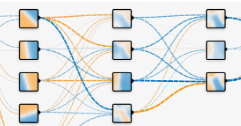
We learned earlier that a Global Average Pooling layer reduces the height-width dimension of a tensor from h x w x d to 1 x 1 x d. A weighted sum is then applied to this 1 x 1 x d dimensional vector/tensor and then fed into a softmax layer to produce the probabilities of the class - the highest probability being the class the model is predicting. If then we can perform a weighted sum on a one-dimensional vector(output of Global Average Pooling layer) to produce another vector(output probabilities) which correctly represents the input image, then perhaps we can perform a weighted sum on a h x w x d tensor, most likely the output of the last convolutional layer or max pool layer to produce a h1 x w1 x d1 tensor which correctly represents the input image also. The output tensor h1 x w1 x d1 contains more spatial information of the input image than the weighted sum of the output of the Global Average Pooling layer. The weights used to perform the weighted sum of the output of the Global Average Pooling layer are the weights corresponding to the predicted class.

We can see from the above image that W1, W2 … Wn are the weights corresponding to the predicted class (Australian terrier). To generate a class activation map for the predicted score, we can map the predicted score back to the last convolutional layer through the weights W1, W2 … Wn. We perform a weighted sum using W1, W2 … Wn on the activations of the last convolutional layer to generate the class activation map.

Now that we have some intuition above how to generate the class activation maps, let’s dive right into code.
Earlier, we state that in order to generate class activation maps, we need to perform a weighted sum on activations of last convolutional layer but in every forward pass, we only get the activation of the last fully connected layer. In order to obtain activation of the last convolutional layer, we use the PyTorch register_forward_hook module. The snippet below illustrates how to do so.
class LayerActivations():
    features=[]
    def __init__(self,model):
        self.hooks = []
        #model.layer4 is the last layer of our network before the Global Average Pooling layer(last convolutional layer).
        self.hooks.append(model.layer4.register_forward_hook(self.hook_fn))
    def hook_fn(self,module,input,output):
        self.features.append(output)
    def remove(self):
        for hook in self.hooks:
            hook.remove()
Whenever we call a forward pass after instantiating the LayerActivations class, the output of model.layer4 is appended to the features list. We can then obtain the output activations by calling LayerActivations(model_ft).features.
model_ft = model.model
acts = LayerActivations(model_ft)
Next we load a test image and perform a forward pass through our model.
loader = transforms.Compose([transforms.Resize((224,224)), transforms.ToTensor()])
def image_loader(image_name):
    image = PIL.Image.open(image_name).convert("RGB")
    image = loader(image).float()
    image = image.unsqueeze(0)
    return image
image_path = '/content/gdrive/My Drive/chest_xray/test/PNEUMONIA/person100_bacteria_475.jpeg'
#load image and perform a forward pass through our model.
img = image_loader(image_path)
logps =  model_ft(img.cuda() if torch.cuda.is_available() else img)
out_features = acts.features[0].squeeze(0) #since we have performed a forward pass through our model, we can obtain activations from layer(model.layer4) defined in the LayerActivation class from the features list and take out the batch dimension.

out_features = np.transpose(out_features.cpu(),(1,2,0)) # Changes shape from 2048 x 7 x7 to 7 x 7 x 2048. Just performs a matrix transpose on the output features tensor.
Printing the size of the output activations of model.layer4(last layer before Global Average Pooling layer), we get 7 x 7 x 2048 as output.We earlier stated that in order to get the class activation map for a particular class, we need to get the weights associated with that class and use that to perform a weighted sum on the activations of the last convolutional layer. Let’s do that in some few lines of code.
ps = torch.exp(logps) #Our final model layer is a log-softmax activation. We perform torch.exp to take out the log and obtain the softmax values.
pred = np.argmax(ps.cpu().detach()) #Obtain the axis of the predicted class.
W = model_ft.fc[0].weight #We obtain all the weights connecting the Global Average Pooling layer to the final fully connected layer.
w = W[pred,:] # We obtain the weights associated with the predicted class which is a 2048 dimensional vector.
Now that we have the activations of the last convolutional layer and the weights associated with the predicted class, we can perform a weighted sum using the np.dot method. A dot function just performs a dot product on two arrays or tensors.
cam = np.dot(out_features.detach(),w.detach().cpu())
#dot product between a 7x7x2048 tensor and a 2048 tensor yields a 7x7 tensor.
#cam will therefore have a shape of 7x7.
From the theories proposed above, cam seems to be our class activation map and yes it is. But cam is a 7x7 tensor which we need to scale up to fit into our image. That is where the Scipy package comes in. Scipy’s ndimg package provides us with a zoom function that we can use to upsample our cam tensor from 7x7 to 224x224 which is the size of our input image. Let’s look at how.
class_activation = ndimg.zoom(cam, zoom=(32,32),order=1)
#zoom is the number of times we scale up our cam tensor. (7x32, 7x32) = (224,224)
Let’s plot both our input image and the class_activation to view our output.
img = np.squeeze(img, axis=0) #removes the batch dimension from the input image (1x3x224x224) to (3x224x224)
img = np.transpose(img,(1,2,0)) #matplotlib supports channel-last dimensions so we perform a transpose operation on our image which changes its shape to (224x224,3)

#we plot both input image and class_activation below to get our desired output.
plt.imshow(img, cmap='jet',alpha=1)  #jet indicates that color-scheme we are using and alpha indicates the intensity of the color-scheme
plt.imshow(class_activation,cmap='jet',alpha=0.5)
And Voila!


Let’s us take a look at some images the model classified as NORMAL.


From these few images, we can observe that the model is looking at a particular area to identify Pneumonia images and completely different area to identify normal images. Now it is safe to say that our model has learnt to distinguish between chest x-ray scans with traces of Pneumonia and those with no traces of Pneumonia.
NEXT STEPS
We’ve just applied deep learning to a very important area currently under research, medical image analysis. We were able to build a powerful model with an insufficient dataset. Stanford researchers recently open sourced their huge chest x-ray dataset which is sufficient enough to build a far more powerful model than what we've built. You may want to try your hands on that alsoLink: https://stanfordmlgroup.github.io/competitions/chexpert/We have focused too much on chest x-ray analysis. You may want to direct your attention on this datasets also by Stanford where bone x-ray scans analyzed for abnormalities.
Link: https://stanfordmlgroup.github.io/competitions/mura/
THANKS TO
- A great thank you to Alexis Cook for her great tutorial on Global Average Pooling and Class Activation Map. https://alexisbcook.github.io/2017/global-average-pooling-layers-for-object-localization/
- Also, I'll like to thank the ML research group at Stanford for such a great and motivating project and also for open sourcing their dataset
ABOUT ME
I am an undergraduate student currently studying Electrical and Electronic Engineering. I am also a deep learning enthusiast and writer. My work mostly focuses on application of computer vision to medical image analysis. I'm hoping to one day break into the field of autonomous vehicles.You can follow along on twitter(@henryansah083): https://twitter.com/henryansah083?s=09 LinkedIn: https://www.linkedin.com/in/henry-ansah-6a8b84167/