The Machine Learning field is growing at a tremendous pace. One of the most interesting aspects of this development is the community created around it. With a closer look, we can see that the ML community can be separated in several niches, interested in different aspects of the discipline. For instance, some are interested in the Mathematics and Statistics behind the learning process...
Introduction
The Machine Learning field is growing at a tremendous pace. One of the most interesting aspects of this development is the community created around it. With a closer look, we can see that the ML community can be separated in several niches, interested in different aspects of the discipline. For instance, some are interested in the Mathematics and Statistics behind the learning process. Others are interested in developing an idea which request the use of ML tools. If you identify yourself as the latter case, you must learn how to use a professional ML library. Among the ML libraries available today, scikit-learn shines as one of the best options.
Scikit-learn is a Python open source library designed to tackle Machine Learning problems from beginning to end. It is used and well praised by big companies like Evernote and Spotify. Moreover, it has tools for all steps of a typical ML workflow. You can use it to load data, separate datasets into train and test sets, perform dimensionality reduction and feature selection, train several well known and well implemented algorithms and fine tune your hyper parameters using model selection. The final result is a robust, efficient and well coded solution for a predictive model. The best part is you will do all of this in a fast development cycle, which Python programmers/developers are used to.
To introduce you to this powerful library, we will build a predictive model to solve the most common and important problem in ML: classification. We will work with a simple ML workflow, where we load some dataset, parse it, pre-process it, fit a model and evaluate the generalization error. Since scikit-learn is not a library specialized in data visualization, we will also use a little bit of pandas and seaborn in some steps of our workflow.
Classification with scikit-learn
Load, parse and visualize data
The first thing we need to start a Machine Learning project is data. More specifically, in our classification problem there is the need of several labeled examples of the pattern to be discovered. The first cool thing about scikit-learn is it already contain a package called sklearn.dataset, which help us in this task. This package has several "toy datasets", which are a great way to get acquainted with handling data and feed them to different ML algorithms. It also has generators of random samples, capable of constructing datasets of arbitrary complexity and size. Finally, there are more advanced capabilities that can help you fetch real datasets used in real world problems.
Since this is our first tutorial using scikit-learn, let's work with the famous iris flower "toy dataset", studied by Fisher in 1936. The dataset has the following properties:
- Basic description: given some morphological measures of a flower, determine it species
- 150 samples
- 3 classes: setosa, versicolor and virginica
- 4 features. All features are real and positive
- 50 samples for each class
To load this dataset into our program and separate it into train and test sets, just type the following code:
from sklearn.datasets import load_iris
from sklearn.model_selection import train_test_split

iris_dataset = load_iris()
X, y = iris_dataset.data, iris_dataset.target
X_train, X_test, y_train, y_test = train_test_split(X, y, test_size=0.25, random_state=31)
Executing the code above, we separate 25 % of the original dataset for the test set, while the rest goes to the train set. Furthermore, we can control the shuffle of the original dataset, specifying the random_state argument .
Now that we have the dataset loaded into our program, it is interesting to take a look in some samples of the data. We could opt to print the numpy ndarray for some of the samples, manipulating X and y directly. However, this a very raw and ugly visualization, so this practice should not be encouraged. A better option is to use the pandas library. For those that don't know it, pandas is a library used for data analysis and it works mainly with tabular data and time series. Let's use it to randomly print out 10 % of our dataset in a adequate tabular visualization.
import numpy as np
import pandas as pd

df = pd.DataFrame(
    data=np.c_[X,y],
    columns=iris_dataset['feature_names'] + ['target'])
df.sample(frac=0.1)
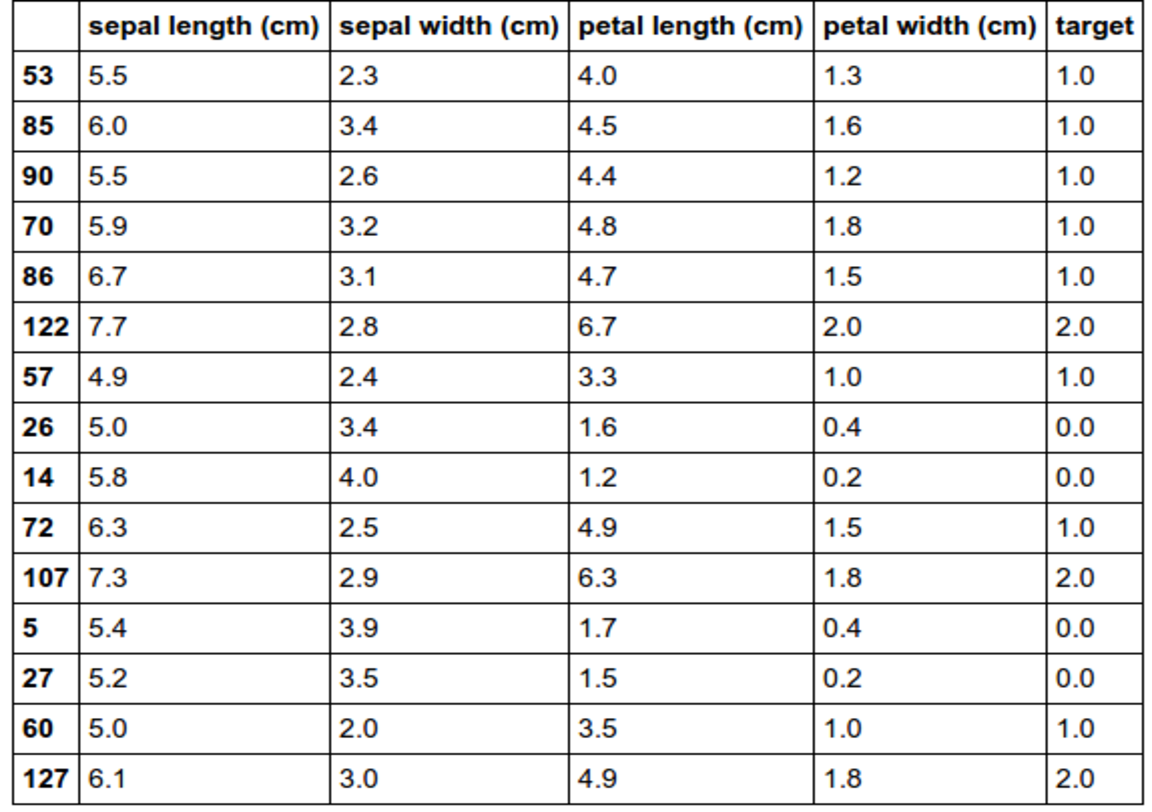
From the table, we can see the features names, units of measure and confirm the properties of the dataset that were mentioned above (4 features, 3 classes, ...). Despite stating the obvious for this "toy dataset", this practice is very useful in real scenarios because we might end up working with a dataset without a detailed description.
Pre-processing stage
Virtually every raw dataset need some pre-processing before we can successfully use it to train ML algorithms (unless someone already did for us). Among common pre-processing tasks are standardization of the features, dimensionality reduction and feature selection. Since we are working with a simple dataset with few features, we will only do the standardization step.
from sklearn import preprocessing

scaler = preprocessing.StandardScaler().fit(X_train)
X_train = scaler.transform(X_train)
X_test = scaler.transform(X_test)
This code guarantees that all features have zero mean and unit variance, a pre-requisite for most ML algorithms to work well.
Training and evaluating generalization
Now comes the most important part of the process: train the machine and test if it has generalized the concept beyond the train set.
This is where scikit-learn shines the most in my opinion. This ML library work with Python objects called estimators, which must implement the methods fit(X, y) and predict(T). That's right, your training is executed in one line of code and all predictions of the test code are made in just one more line! For evaluating the generalization of our machine, we use one of the metrics defined in the package sklearn.metrics. The code below show an example, where we train a Support Vector Machine to classify our data using the accuracy score.
from sklearn import svm
from sklearn.metrics import accuracy_score

clf = svm.SVC(gamma=0.001, C=100.)
clf.fit(X_train, y_train)
y_pred_train = clf.predict(X_train)
y_pred_test = clf.predict(X_test)
acc_train = accuracy_score(y_train, y_pred_train)
acc_test = accuracy_score(y_test, y_pred_test)
In the code above we trained a SVM with a set of fixed hyper parameters gamma and C. This should give us accuracies of about 97 % for the training and test set, which are great results. To obtain more details about the performance of our machine we can calculate and visualize the confusion matrix. And, as you might have suspected, scikit-learn also has a function to calculate the matrix for us.
#If you are using a Jupyter notebook, use the magic command    below. Else, ignore it.
%matplotlib inline
from sklearn.metrics import confusion_matrix
import matplotlib.pyplot as plt
import seaborn as sns

confusion_matrix = confusion_matrix(y_test,y_pred_test) # Returns a ndarray
cm_df = pd.DataFrame(
    confusion_matrix,
    index = [idx for idx in ['setosa', 'versicolor', 'virginica']],
    columns = [col for col in ['setosa', 'versicolor', 'virginica']])
plt.figure(figsize = (10,7))
sns.heatmap(cm_df, annot=True)
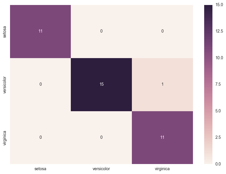
In the code above, again we use the power of pandas, together with the visualization library seaborn to produce a beautiful and detailed visualization of our results in the test set. From the confusion matrix we can see that the only mistake was one versicolor that was mistaken as a virginica.
So, we have finished training our first machine in scikit-learn. Congratulations! But don't think this is the end. On the contrary, there is a huge amount of modules to discover, change and combine in your workflow to obtain new and better results. Also, since the library is open source, we can even read the code and alter it to target a specific dataset. One possible change we could make in our model is to switch the estimator and use Fisher Linear Discriminant Analysis instead of SVM. This change can be made in a few line of codes:
from sklearn.discriminant_analysis import LinearDiscriminantAnalysis

clf = LinearDiscriminantAnalysis()
clf.fit(X_train, y_train)
Using the predict method, we should end up with accuracy of about 98 % for the train set and 97 % for the test set. It is not easy to get better results that those ones. Nonetheless, if you want to try to reach the 100 %, the next step would be hyper parameter tuning. This would require separating one more set for validation of the hyper parameters or using cross validation. And yes, scikit-learn also have this figured out for you.
Conclusion
In this tutorial, you were introduced to a Python Machine Learning library known as scikit-learn. Along the tutorial you learned that scikit-learn:
- is a open source ML library praised by professionals and big companies.
- is capable of assist you in most of the problems you're going to face when constructing predictive models
- gives solutions in few lines of code
- should be paired with data analysis and data visualization libraries to get the most of it
- has several modules which should be experimented, concatenated, and changed in the pursuit of the bests results
For next steps, you should head to the examples page in the scikit-learn webpage and get some inspirations. You can also browse through its quick-start, tutorials and user guide pages to get a more broader view of everything the library has to offer. For those more interested in deep learning, you should be aware that scikit-learn don't has the requirements to create serious deep learning neural networks. However, there is a project called skflow which gives TensorFlow a scikit-learn interface.
To get started with your own ML-in-a-box or data science setup, sign up here.

