Predictive Analysis for Sales: A Comprehensive Forecasting Approach 📈🕵🏼‍♂️👨🏼‍💻

Machine Learning (ML) is a powerful tool to predict sales or understand the behavioral pattern underlying the data. In an era where data is the fuel to transform any business and revolutionize its sales strategies, at the forefront of this transformation is predictive analysis empowered by the capabilities of machine learning. This dynamic combination not only enables organizations to make sense of vast datasets but also empowers them to forecast sales trends, optimize decision-making, and ultimately drive revenue growth.

Machine learning algorithms can be trained to recognize patterns and correlations within the data, enabling organizations to predict future outcomes with a high degree of accuracy. Whether it's forecasting customer demand, identifying high-value leads, or optimizing pricing strategies, predictive analysis driven by machine learning provides a data-driven foundation for decision-makers.

In this article, we will try to forecast the sales of a store using Kaggle's dataset. The main objective of this challenge is to create an ML model to predict the sales data for future months.

Sales forecasting involves the estimation of future sales using predictive models or adapted methods, with varying degrees of accuracy. This practice necessitates the consideration of both qualitative and quantitative variables in the process.

Sales forecasting involves understanding the pattern of business by using technology such as ML. This involves creating a model which takes in large amount of historical data on which future patterns are predicted.

Understanding the Significance of Future Sales Forecasting

Sales forecasting plays a crucial role in businesses decision making by providing insights into what to expect from the coming months. Here are a few key points to understand why sales forecasting is useful in business:

• Strategic Decision Making: Sales forecasting aids in strategic decision-making by providing insights into expected sales. This in turn helps any business to be prepared by setting up realistic goals, allocating adequate resources, and planning for growth.
• Marketing Strategy: Forecasting generates critical data for businesses. This information can help in making strategic decisions such as allocating marketing budgets effectively, directing efforts toward the appropriate target audience, and evaluating the future sales impact of marketing campaigns.
• Financial Planning: Future sales forecasts contribute to effective financial planning. Businesses can align their budgets with expected revenue, manage cash flow, and make informed financial decisions.
• Risk Management: Forecasting allows businesses to identify potential risks and uncertainties. By understanding market dynamics, businesses can develop strategies to mitigate risks associated with economic fluctuations, changing consumer behavior, or external factors.

Challenges

Sales forecasting addresses the performance and profitability requirements of organizations, making it a crucial element in a company's sales strategy, irrespective of its industry or sector. When discussing the strategic aspects of sales forecasting, we are essentially focusing on the challenges that, if resolved, would enable a company to implement its sales strategy with greater confidence.

• Market Uncertainty: Market conditions are often unpredictable, making it challenging to accurately forecast sales. External factors such as geopolitical events, economic downturns, or natural disasters can significantly impact consumer behavior.
• Seasonal Variations: Many industries experience seasonal fluctuations in demand. Forecasting becomes complex when dealing with the cyclical nature of certain products or services, requiring businesses to account for these variations.
• Changing Consumer Behavior: Rapid changes in consumer preferences and behavior can disrupt traditional forecasting models. Shifts in buying patterns influenced by technological advancements or cultural changes pose challenges for accurate predictions.
• Competitive Dynamics: The competitive landscape is dynamic, with new entrants, evolving strategies, and changing market shares. Predicting the actions of competitors and their impact on sales adds an additional layer of complexity.

Different Machine Learning Methods for Sales Forecasting

Here are some common machine learning methods used in sales forecasting:

• Linear Regression: Linear regression models establish a linear relationship between the input features and the target variable (sales). It is suitable for scenarios where the relationship is expected to be approximately linear.
• Time Series Analysis: Time series methods, such as ARIMA (AutoRegressive Integrated Moving Average) or Exponential Smoothing, are specifically designed for forecasting based on historical time-ordered data. These methods consider patterns and seasonality in the time series.
• Decision Trees: Decision trees are tree-like models that split data based on input features, creating a set of rules for predicting the target variable. They are intuitive and can handle both numerical and categorical data.
• Random Forest: Random Forest is an ensemble method that builds multiple decision trees using random feature selection with replacement and combines their predictions. It often performs well and is robust to overfitting.
• Neural Networks (Deep Learning): Neural networks, especially deep learning models, can capture complex patterns in data. Recurrent Neural Networks (RNNs) and Long Short-Term Memory networks (LSTMs) are commonly used for sequential data like time series.
• K-Nearest Neighbors (KNN): KNN is a simple algorithm that classifies data points based on the majority class of their nearest neighbors. It can be adapted for regression tasks in sales forecasting.
• XGBoost: XGBoost is an efficient and scalable implementation of gradient boosting. It is particularly effective in handling large datasets and has been successful in various machine learning competitions.
• Ensemble Methods: Ensemble methods, including bagging and boosting, combine multiple models to improve overall performance. Bagging methods like Bootstrap Aggregating (Bagging) and boosting methods like AdaBoost are commonly used.

It is common to experiment with multiple methods to determine which one performs best for a particular scenario.

Sales Forecasting Using Python on the Paperspace Platform

Here we will try to use a Kaggle's sales dataset and use various ML techniques to predict the sales for future data. We have provided the CSV for the reader's convenience.

Please click the link to access the entire notebook and access the full code. In this article we are providing a comprehensive code overview.

1. Importing the necessary libraries

#import the libraries
import pandas as pd
import numpy as np
from sklearn.model_selection import RandomizedSearchCV
import joblib
import os
import matplotlib.pyplot as plt
import seaborn as sns
import warnings
import pickle

from sklearn.linear_model import LinearRegression
from sklearn.ensemble import RandomForestRegressor
import xgboost as xgb
from sklearn.metrics import mean_absolute_error, mean_squared_error, r2_score
warnings.filterwarnings('ignore')

# settings to display all columns
pd.set_option("display.max_columns", None)

2. Loading and Exploration of the Data

Let us start by loading the datasets to perform the basic Exploratory Data Analysis (EDA) on the data.

#function that will be used for the extraction of a CSV file and then converting it to pandas dataframe
def load_data(file_name):  
    """Returns a pandas dataframe from a csv file."""  
    return pd.read_csv(file_name)
train_df = load_data('train.csv')
test_df = load_data('test.csv')
syb_df = load_data('sample_submission.csv')

The below piece of code provides the time period of the available data, provided for the model training and testing data

def sales_period(data):  
    """Time interval of train dataset:"""  
  
    print(f'time period starts from :{data["date"].min()}, and ends in :{data["date"].max()}')
sales_period(train_df)
sales_period(test_df)

time period starts from :2013-01-01, and ends in :2017-12-31
time period starts from :2018-01-01, and ends in :2018-03-31

3. Basic EDA

def sales_per_store(data):
    
    sales_by_store = data.groupby('store')['sales'].sum().reset_index() 
    fig, ax = plt.subplots(figsize=(8,6)) 
    sns.barplot(sales_by_store, x="store", y="sales", estimator="sum", errorbar=None)
    ax.set(xlabel = "Store Id", ylabel = "Sum of Sales", title = "Total Sales Per Store")   
     
    return sales_by_store, ax

sales_per_store(train_df)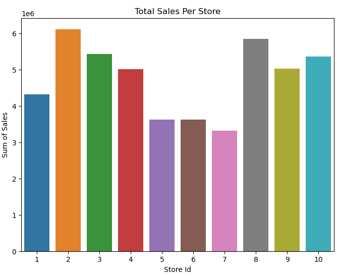

def sales_by_dt(data):
    data['date'] = pd.to_datetime(data['date'])
    sales_by_date = data.groupby('date')['sales'].sum().reset_index()

    #display the results
    return sales_by_date

sales_by_date = sales_by_dt(train_df)

Plot the sales to understand the sales pattern over time

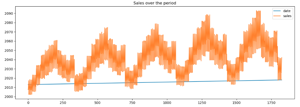
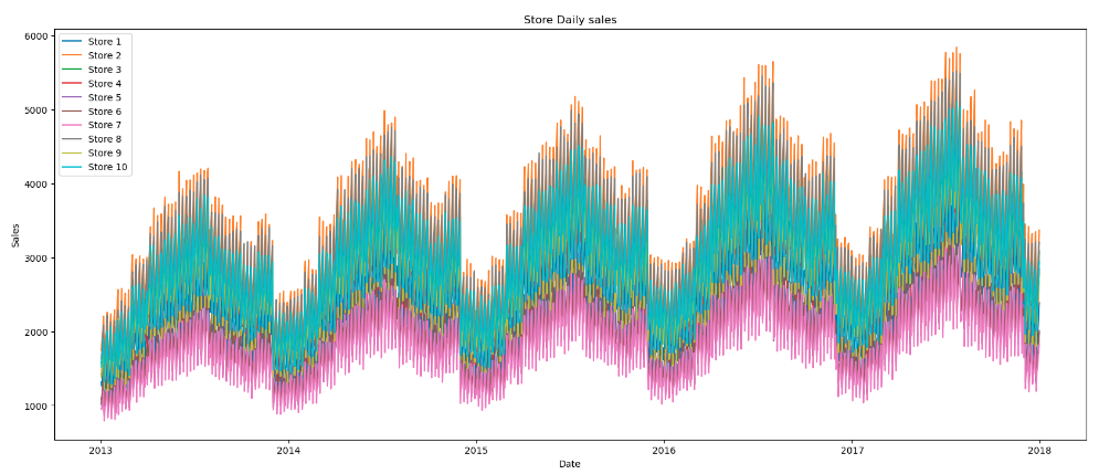
As evident from the plot we notice that the sales have increased over the years for all the stores.

4. Data Preprocessing along with EDA at each step

The below code snippet takes the original training DataFrame (train_df), groups the data by date, sums the sales for each date, converts the index to datetime format, drops unnecessary columns. This transformation is useful when analyzing overall sales trends on a daily basis, without considering individual stores or items.

#Aggregate Daily Sales Data by Date from Training Dataset
train_dt_sales = train_df.groupby('date').sum('sales')
train_dt_sales.index = pd.to_datetime(train_dt_sales.index)
train_dt_sales = train_dt_sales.drop(['store','item'], axis=1)
train_dt_sales.head()

DataFrame is split into two parts: the training set (train) and the test set (test). In this case, all data before January 1, 2017, is considered the training set, while data from and after January 1, 2017, is considered the test set.

#creates a train/test split of time series data, plots the training and test sets on a single graph, and adds a visual indicator of the split point
train = train_dt_sales.loc[train_dt_sales.index < '01-01-2017']
test = train_dt_sales.loc[train_dt_sales.index >= '01-01-2017']

fig, ax = plt.subplots(figsize=(15, 5))
train.plot(ax=ax, label='Training Set', title='Train/Test Split data')
test.plot(ax=ax, label='Test Set')
ax.axvline('01-01-2017', color='Gray', ls='--')
ax.legend(['Training Set', 'Test Set'])
plt.show()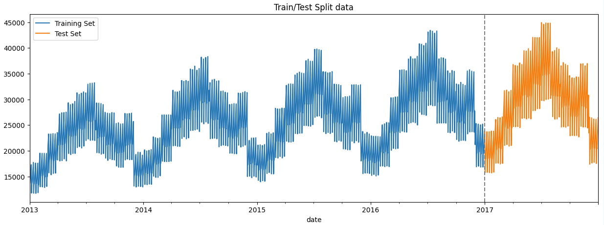

In the dataset we are provided with the date column which can be used to extract features such as 'day_of_week', 'day_of_year', 'quarter', etc.

#creating features from the existing features such as day of week, hour, month
def create_features(df):
    """
    Creating time series features based on dataframe index.
    """
    df = df.copy()
    # df['hour'] = df.index.hour
    df['dayofweek'] = df.index.dayofweek
    df['quarter'] = df.index.quarter
    df['month'] = df.index.month
    df['year'] = df.index.year
    df['dayofyear'] = df.index.dayofyear
    df['dayofmonth'] = df.index.day
    df['weekofyear'] = df.index.isocalendar().week
    return df

train_dt_sales = create_features(train_dt_sales)

The below plots helps to analyse the sales data over the week and month

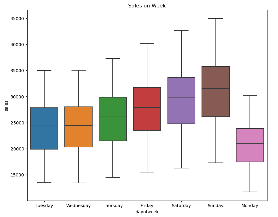
Sales typically exhibit an upward trend starting from Friday, reach their peak on Sunday, and then experience a decline on Monday. This pattern is influenced by the increased sales that commonly occur over the weekends.

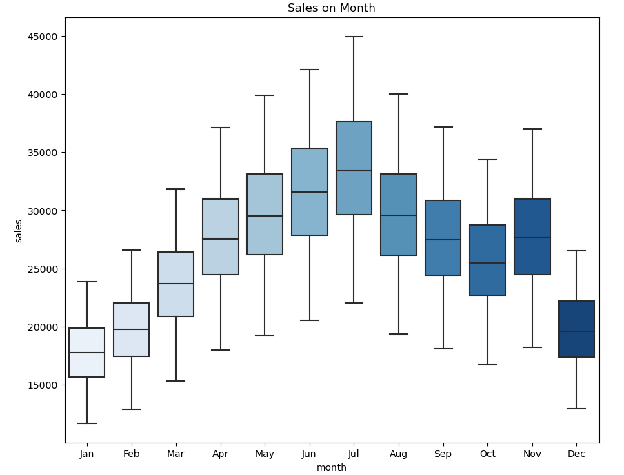
In the plot above we notice that a strong shift occurs from the month of April and starts declining from August. Furthermore, the plot shows an upward spike in the month of November.

5. Model building

We aim to employ three distinct models—Linear Regression, Random Forest, and XGBoost—to forecast sales using the training dataset. The best model among these will be utilized to predict sales for the test data.

Let us start with building a linear regression model to predict the sales.

Linear Regression

Linear regression is a supervised ML algorithm that provides a linear relationship between a dependent and an independent variable by drawing a best fit line between the two variables.

# fit a linear regression model
linreg_model = LinearRegression()
linreg_model.fit(X_train, y_train)

#predict on the test(future) data
test['prediction_lr'] = linreg_model.predict(X_test)

The below code calculates and prints three performance metrics to evaluate the performance of a Linear Regression model on the test data.

#metrics to verify the model
linreg_rmse = np.sqrt(mean_squared_error(test['sales'], test['prediction_lr']))
linreg_mae = mean_absolute_error(test['sales'], test['prediction_lr'])
linreg_r2 = r2_score(test['sales'], test['prediction_lr'])
print('Linear Regression RMSE: ', linreg_rmse)
print('Linear Regression MAE: ', linreg_mae)
print('Linear Regression R2 Score: ', linreg_r2)

Root Mean Squared Error (RMSE): The mean_squared_error function from sklearn.metrics is used to calculate the mean squared error between the actual sales (test['sales']) and the predicted sales (test['prediction_lr']) by the Linear Regression model. The result is then square-rooted to obtain the RMSE.

Mean Absolute Error (MAE): The mean_absolute_error function is used to calculate the mean absolute error between the actual and predicted sales. It provides the average absolute difference between the predicted and actual values.

R-squared (R2) Score: The r2_score function calculates the R-squared score, which indicates the proportion of the variance in the dependent variable (sales) that is predictable from the independent variable (prediction_lr). It measures the goodness of fit of the model.

Random Forest

Random Forest is an ensemble learning method used for both classification and regression tasks in machine learning. Random Forest builds multiple decision trees during training. Each tree is trained on a random subset of the features and a random subset of the training data. This randomness helps prevent overfitting and contributes to the model's robustness.

# biuld a random forest model 
rf_model = RandomForestRegressor(n_estimators=100, max_depth=20)
rf_model.fit(X_train, y_train)

test['prediction_rf'] = rf_model.predict(X_test)
#model evaluation metrics
rf_rmse = np.sqrt(mean_squared_error(test['sales'], test['prediction_rf']))
rf_mae = mean_absolute_error(test['sales'], test['prediction_rf'])
rf_r2 = r2_score(test['sales'], test['prediction_rf'])
print('Random Forest RMSE: ', rf_rmse)
print('Random Forest MAE: ', rf_mae)
print('Random Forest R2 Score: ', rf_r2)

The provided code snippet builds a Random Forest model for regression using the RandomForestRegressor from scikit-learn.

XGBoost

XGBoost, short for eXtreme Gradient Boosting, is a powerful and widely used machine learning algorithm that belongs to the gradient boosting family. It is particularly popular for its high performance, efficiency, and versatility in a variety of machine learning tasks, including classification, regression, and ranking problems.

# xgboost model 

reg = xgb.XGBRegressor(base_score=0.5, booster='gbtree',    
                       n_estimators=1000,
                       early_stopping_rounds=50,
                       objective='reg:linear',
                       max_depth=3,
                       learning_rate=0.01)
reg.fit(X_train, y_train,
        eval_set=[(X_train, y_train), (X_test, y_test)],
        verbose=100)

xg_rmse = np.sqrt(mean_squared_error(test['sales'], test['prediction_xg']))
xg_mae = mean_absolute_error(test['sales'], test['prediction_xg'])
xg_r2 = r2_score(test['sales'], test['prediction_xg'])
print('Random Forest RMSE: ', xg_rmse)
print('Random Forest MAE: ', xg_mae)
print('Random Forest R2 Score: ', xg_r2)

Results

When comparing various machine learning models, it's important to consider several factors for comparison.

In our specific case, we will specifically focus on evaluating models using the Root Mean Squared Error (RMSE), Mean Absolute Error (MAE), and R-squared (R2) Score.

In our case, we will use a random forest model to predict the sales for the test data.

# drop the unnecessary columns and biuld the model
test_df.drop(['id','store','item'], axis=1, inplace=True)
test_df.index = pd.to_datetime(test_df.date)
to_predict_test_feature = create_features(test_df)
to_predict_test_feature = to_predict_test_feature[FEATURES]
to_predict_test_feature['prediction'] = reg.predict(to_predict_test_feature)
to_predict_test_feature.head()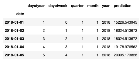

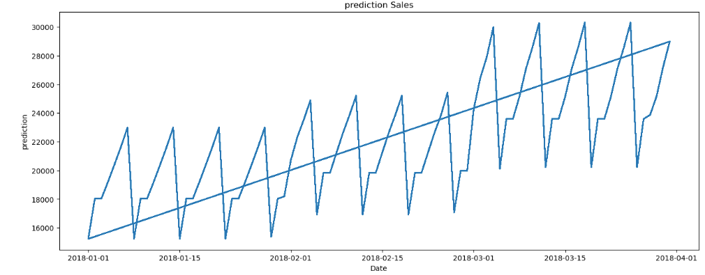
Plot the sales prediction

Conclusion

In this tutorial, we utilized the capabilities of machine learning for sales forecasting, a slightly different approach from conventional methods like the ARIMA model. Nonetheless, this approach proves highly effective in accurately predicting sales. The utilization of advanced algorithms, such as XGBoost and Random Forest, enables businesses to extract valuable insights from vast datasets, enhancing their predictive capabilities. The significance of accurate sales forecasting extends beyond mere numerical predictions; it becomes a strategic tool that empowers organizations to optimize resource allocation, refine marketing strategies, and fortify decision-making processes.

We strongly encourage you to execute the notebook and explore its functionalities. Our intention is to build a strong foundation framework for the model and its experiments, serving as a starting point for your exploration.

Thank you so much for reading!!

References

• Dataset Link:- https://www.kaggle.com/competitions/demand-forecasting-kernels-only
• Code Reference:- https://www.javatpoint.com/sales-prediction-using-machine-learning
• Challenges of Sales Forecasting:- https://www.verteego.com/en/what-are-the-challenges-of-sales-forecasting