CVPR 2020 brought its fair share of novel ideas in the domain of Computer Vision, along with a number of interesting ideas in the field of 3D vision. Among all these new ideas explored, a notable paper authored by researchers at Huawei, University of Sydney and Peking University titled GhostNet: More Features from Cheap Operations managed to turn some heads. The idea, despite being fairly simple, was able to achieve competitive and interesting results.
This article will start by covering the fundamentals behind feature maps in convolutional neural networks, and we will observe a general pattern in these maps which are central to the performance of a CNN. We will then do a review of GhostNet and an in-depth analysis of its capabilities and shortcomings.
Table of Contents:
- Convolution
- Feature Map Pattern Redundancy
- GhostNet
- Depthwise Convolution
- Code
- Results
- Shortcomings
- References and Further Reading
Bring this project to life
Convolution
Before we dive into the concepts governing GhostNet, it's imperative to do a brief recap of the convolution algorithm. Readers with a strong understanding of the convolution algorithm used in standard convolutional neural network architectures should feel free to skip this section. For a more formal introduction and in-depth dissection of convolution, the article titled A guide to convolution arithmetic for deep learning is a great place to start. Here we'll just review enough to have the required knowledge to understand GhostNet.
To summarize, convolution is the most fundamental process involved in any convolutional neural network (CNN). Drawing its roots from foundational signal and image processing, convolution is a simple process of filtering an image using a kernel to propagate certain texture-based information of the original image.
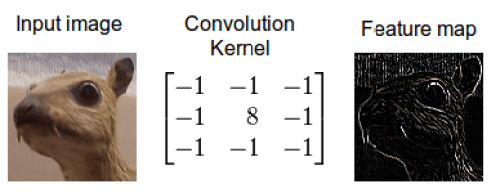
In image processing, to understand the semantics of an image, it's critical to either enhance or preserve certain texture-based information which is easier to process using algorithms. Traditional techniques involve detecting edges of objects in images, outlining contours, finding corner points, etc. The evolution of computer vision (and deep learning in general) provided algorithms with the capability to learn these features in the input image using trainable convolutional kernels, which formed the basis of convolutional neural network architectures.
These filters/kernels, also termed as "weight matrices", contain numerical values which are applied to the input image and are tuned by back-propagation to capture intrinsic internal feature representations of the given input image. In general terms, a convolutional layer takes an input tensor of C channels and outputs a tensor of C' channels. These C' channels are determined by the number of filters/kernels present in that layer.
Now that we have gone through the background check on convolution in deep CNNs, let's understand the foundation of the GhostNet paper: Feature Maps.
Feature Map Pattern Redundancy
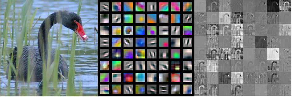
Feature Maps are spatial maps generated from an input by applying a standard convolutional layer. These feature maps are responsible for preserving/propagating certain feature-rich representations of the input image based on the learned convolutional filter weights for that layer.
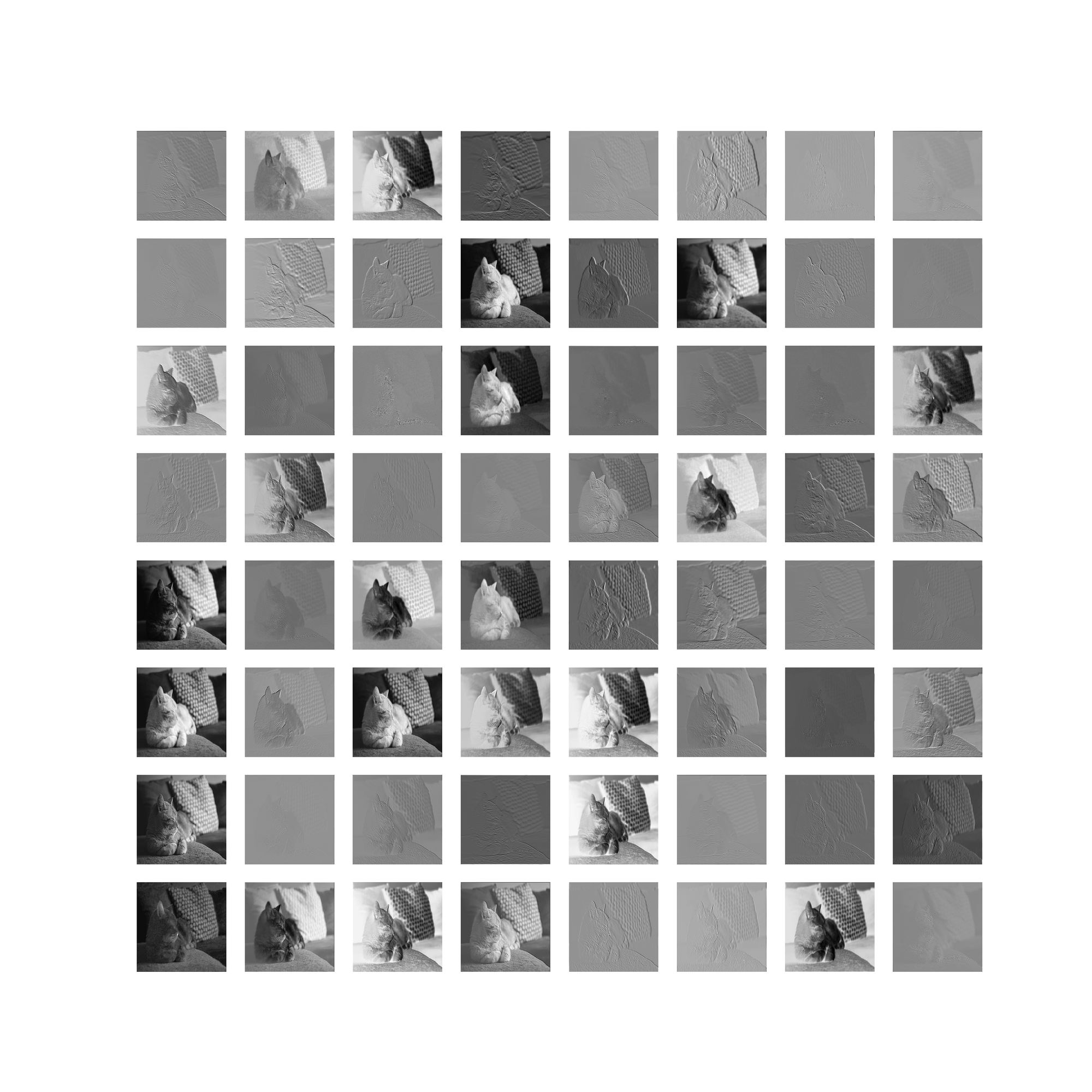
The authors of GhostNet analyzed feature maps in standard convolutional layers to see whether they exhibit a certain pattern or not. Upon investigation, they noticed that in the whole set of feature maps generated by the convolutional layer, there exist many similar copies of unique intrinsic feature maps which become redundant to generate from the rather expensive convolutional operation. As one can observe from the set of feature maps shown in the above image, there exist several similar-looking copies, like those in the 6th row, 1st and 3rd columns.
The authors coin the term "Ghost Feature Maps" to refer to these redundant copies. This serves as the motivating foundation for the paper: how can we reduce the computation involved in generating these redundant feature maps?
GhostNet
Reducing parameters, reducing FLOPs, and getting near-baseline accuracy is an absolute win-win-win situation. This was the motivation for the Huawei Noah Ark Lab's work on GhostNet, published at CVPR-2020. Although the approach might look complicated at first glance, it is fairly straightforward and easy to interpret and validate. The paper aims to provide a cheaper alternative to natural convolutional layers used in standard deep convolutional neural networks.
So what's the idea?
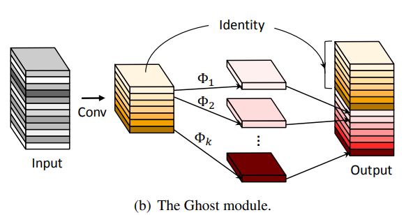
As we saw before, a convolutional layer takes in an input tensor defined by the number of input channels, C, and outputs a tensor of C' channels. These channels are essentially the feature maps discussed above, and as we saw there exist redundant copies of these feature maps in that set. Instead of creating all of the feature maps by standard convolution, what GhostNet does is to generate x% of the total output feature maps, while the remaining are created by a cheap linear operation. This cheap linear operation results in a massive reduction in parameters and FLOPs, while retaining nearly the same performance as that of the original baseline model. The cheap linear operation is designed in such a way that it resembles the characteristics of intrinsic convolution, and usually should be learnable and input-dependent, so that it can be optimized in the backward pass using backpropagation.
Before we discuss the exact linear operation/transformation used in GhostNet, let's take a second to note other similar ideas for inducing sparsity in neural networks, or making them more efficient. There have been several approaches for pruning neural networks suggested recently which significantly reduce the complexity of deep neural networks. However, most of these methods can only be incorporated post-training, i.e, after the original deep model has been trained. Thus, they serve mostly the purpose of compressing trained models to the smallest size while preserving their performance.
One of the prominent ideas in this area, also known as Filter Pruning, is done via a simple process. Once the model is trained, the trained filters in any layer of the model are obtained, and the corresponding absolute sum of the weights in those filters are calculated. Only the top-x filters with higher absolute weights' sums are preserved, while the remaining filters are discarded.
Now, back to the "cheap linear transformation" in GhostNet. The paper uses Depthwise convolution (often denoted as DWConv) as its cheap linear transformation. We discussed what convolution is in the preceding sections. So, what is Depthwise Convolution (DWConv)?
Depthwise Convolution
Convolution serves as the holy grail of standard deep neural network architectures, used predominantly in computer vision-based problems. However, convolution does have certain shortcomings which have been addressed in many works over the years. Some include adding a structural prior to the filters/kernels used in the convolutional layers so they're contextually adaptive. Others include changing the architectural process governing a convolution operation. Usually in deep neural networks, the convolutional layers receive inputs from the activation of the previous output, which is a 4-dimensional tensor denoted as (B, C, H, W), also called channel-first format (else in (B, H, W, C) format). Here, B represents the batch size used while training; H and W represent the spatial dimensions of the input, i.e., the height and width of the input feature map, and finally C denotes the number of channels in the input tensor. (Note: TensorFlow usually follows the latter format for specifying the dimension of tensors: (N, H, W, C), where N is the same as B, i.e. batch size. PyTorch uses the channel-first format as standard practice). Thus, while computing multi-channel intrinsic convolution, the filters (which are of the same depth as the input) are applied on the input tensor to produce the required number of output channels. This increases complexity in correspondence to both the number of input channels and the number of output channels.

Depthwise convolution was introduced to address this issue of high parameters and FLOPs induced by normal convolution. Instead of applying the filters on all the channels of the input to generate one channel of the output, the input tensors are sliced into individual channels and the filter is then applied only on one slice; hence the term "depthwise", which basically means per-channel convolution. In simple terms, a 2D filter/kernel/window is convolved with one channel which is a two-dimensional slice to output one channel (also 2-D) for the output tensor for that layer. This reduces the linearly increasing computational overhead in natural convolutions. However, there is a caveat: for depthwise convolutions to provide the incremental speed and lower complexity, the number of channels in the input tensor and the resultant output tensor in the particular layer should match. Thus, it's a two-fold process: 1. Convolve 2-D filters with each channel of the input tensor to generate the 2-D output channels, then 2. Concatenate/stack these 2-D channels to complete the output tensor. (For further reading on the different types of convolutions and in-depth analysis on them, I recommend going through this article).
Depthwise convolutions thus result in heavy parameter reduction and reduced operations, making it cheap to compute while maintaining a close relationship with intrinsic convolution. This is the "magic" behind GhostNet's performance. Although the authors don't explicitly mention in their paper that Depthwise convolution serves as the cheap linear transformation, it's purely a design choice. This question was even raised in this GitHub issue on the official repository for the paper.
GhostNet therefore proposes an essentially standalone replacement layer for standard convolution layers in deep neural network architectures, where the output tensor for any convolutional layer is now created by a serialization of two operations. First, generate x% of the total channels for the output tensor by a sequential stack of three layers: standard convolution followed by batch normalization and a non-linear activation function, which is defined to be Rectified Linear Unit (ReLU) by default. The output of this is then passed to the secondary block, which is again a sequential stack of three layers: depthwise convolution followed by batch normalization and ReLU. Finally, the tensor from the first sequential block is stacked with the output from the secondary sequential block to complete the output tensor.
Let's understand this by a simple set of mathematical steps:
Assume x is the input tensor of dimension (B, C, H, W) for a particular convolutional layer in a deep neural network architecture. The output for the layer is expected to be x1 of dimension (B, C1, H1, W1). The following operations define a Ghost convolution used in place of a standard convolution:
Step 1 (Primary Convolution): Compute f(x) on the input tensor x to generate a tensor of dimension (B, C1/2, H1, W1) where f(x) represents standard convolution plus batch normalization plus ReLU. This new tensor can be denoted as y1.
Step 2 (Secondary Convolution): Compute g(x) on the tensor y1 to generate a tensor of dimension (B, C1/2, H1, W1) where g(x) represents depthwise convolution plus batch normalization plus ReLU. This new tensor can be denoted as y2.
Step 3 (Stack): Stack/concatenate y1 and y2 to form the resultant output tensor x1.
In the above steps, we fixed the amount of feature maps to be generated by both the primary and secondary block to be 50% each of the total output feature maps the tensor is supposed to have. However, the layer is flexible to compute at a different ratio. 50% reflects a parameter for the layer, denoted by s, with a default value of 2. Usually the paper records observations at this ratio (referred to as "ratio 2"), however upon increasing the ratio the parameters can be further reduced with a trade-off between speed and accuracy. Higher values for s essentially means more feature maps are computed by the depthwise kernel, rather than by the standard convolution in the primary block. This translates to larger model compression and increased speed, but lower accuracy.
The authors performed ablation experiments on different kernel sizes for the depthwise convolution filters. The results are discussed in the section below, GhostNet Results.
The authors also proposed a new backbone architecture called GhostNet, which is essentially a MobileNet v3 where the bottleneck is replaced by a Ghost Bottleneck. Ghost modules essentially form the foundation of these Ghost Bottlenecks, which follow the same architectural structure as that of a standard MobileNet v3 bottleneck.
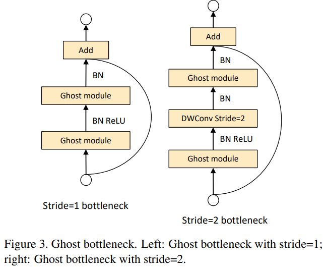
GhostNet is built by stacking these ghost bottlenecks with increasing channels in the tensor in a series after the input layer, which is a standard convolutional layer. (Note: The input convolutional layer, often referred to as the stem of the model, wasn't replaced with a Ghost convolution block). The ghost bottlenecks are grouped together in stages based on the input feature map dimensionality. All the ghost bottlenecks were applied with stride of 1, except for the last bottleneck where the stride 2 design was used, as shown in the above diagram. For some residual connections in the Ghost bottlenecks the authors even used Squeeze-Excitation (SE) blocks to provide channel attention, thus improving accuracy with a small computational overhead.
GhostNet Code
Let's dive into the code for both the Ghost block and the Ghost Bottleneck which can be simply integrated into any baseline convolutional neural networks.
We'll start with the PyTorch and TensorFlow-based code for Ghost Convolution, which can be used as a direct swap for standard convolutional layers.
Ghost Convolution (PyTorch)
### Import necessary libraries and dependencies
import torch
import torch.nn as nn
import math

class GhostModule(nn.Module):
    def __init__(self, inp, oup, kernel_size=1, ratio=2, dw_size=3, stride=1, relu=True):
        super(GhostModule, self).__init__()
        self.oup = oup
        ### Compute channels for both primary and secondary based on ratio (s)
        init_channels = math.ceil(oup / ratio)
        new_channels = init_channels*(ratio-1)

		### Primary standard convolution + BN + ReLU
        self.primary_conv = nn.Sequential(
            nn.Conv2d(inp, init_channels, kernel_size, stride, kernel_size//2, bias=False),
            nn.BatchNorm2d(init_channels),
            nn.ReLU(inplace=True) if relu else nn.Sequential(),
        )

		### Secondary depthwise convolution + BN + ReLU
        self.cheap_operation = nn.Sequential(
            nn.Conv2d(init_channels, new_channels, dw_size, 1, dw_size//2, groups=init_channels, bias=False),
            nn.BatchNorm2d(new_channels),
            nn.ReLU(inplace=True) if relu else nn.Sequential(),
        )

    def forward(self, x):
        x1 = self.primary_conv(x)
        x2 = self.cheap_operation(x1)
        ### Stack
        out = torch.cat([x1,x2], dim=1)
        return out[:,:self.oup,:,:]
GhostNet Convolution (TensorFlow)
### Import necessary dependencies and libraries
import tensorflow as tf
from tensorpack.models.common import layer_register
from tensorpack.utils.argtools import shape2d, shape4d, get_data_format
from tensorpack.models import BatchNorm, BNReLU, Conv2D
import math
import utils

### Depthwise convolution kernel weight initializer
kernel_initializer = tf.contrib.layers.variance_scaling_initializer(2.0)

### Secondary Depthwise Convolution layer
@layer_register(log_shape=True)
def MyDepthConv(x, kernel_shape, channel_mult=1, padding='SAME', stride=1, rate=1, data_format='NHWC',
              W_init=None, activation=tf.identity):
    in_shape = x.get_shape().as_list()
    if data_format=='NHWC':
        in_channel = in_shape[3]
        stride_shape = [1, stride, stride, 1]
    elif data_format=='NCHW':
        in_channel = in_shape[1]
        stride_shape = [1, 1, stride, stride]
    out_channel = in_channel * channel_mult

    if W_init is None:
        W_init = kernel_initializer
    kernel_shape = shape2d(kernel_shape) #[kernel_shape, kernel_shape]
    filter_shape = kernel_shape + [in_channel, channel_mult]

    W = tf.get_variable('DW', filter_shape, initializer=W_init)
    conv = tf.nn.depthwise_conv2d(x, W, stride_shape, padding=padding, rate=[rate,rate], data_format=data_format)
    if activation is None:
        return conv
    else:
        return activation(conv, name='output')


def GhostModule(name, x, filters, kernel_size, dw_size, ratio, padding='SAME', strides=1, data_format='NHWC', use_bias=False,
                activation=tf.identity):
    with tf.variable_scope(name):
        init_channels = math.ceil(filters / ratio)

        ### Primary standard convolution
        x = Conv2D('conv1', x, init_channels, kernel_size, strides=strides, activation=activation, data_format=data_format,
                   kernel_initializer=kernel_initializer, use_bias=use_bias)
        if ratio == 1:
            return x #activation(x, name='output')
        dw1 = MyDepthConv('dw1', x, [dw_size,dw_size], channel_mult=ratio-1, stride=1, data_format=data_format, activation=activation)
        dw1 = dw1[:,:,:,:filters-init_channels] if data_format=='NHWC' else dw1[:,:filters-init_channels,:,:]

        ### Stack
        x = tf.concat([x, dw1], 3 if data_format=='NHWC' else 1)
        return x
Now let's take a look at the PyTorch implementation of the Ghost Bottleneck, which is used as the building blocks for GhostNet.
Ghost Bottleneck (PyTorch)
### Squeeze Excitation Block
class SELayer(nn.Module):
    def __init__(self, channel, reduction=4):
        super(SELayer, self).__init__()
        self.avg_pool = nn.AdaptiveAvgPool2d(1)
        self.fc = nn.Sequential(
                nn.Linear(channel, channel // reduction),
                nn.ReLU(inplace=True),
                nn.Linear(channel // reduction, channel),        )

    def forward(self, x):
        b, c, _, _ = x.size()
        y = self.avg_pool(x).view(b, c)
        y = self.fc(y).view(b, c, 1, 1)
        y = torch.clamp(y, 0, 1)
        return x * y


### DWConv + BN + ReLU
def depthwise_conv(inp, oup, kernel_size=3, stride=1, relu=False):
    return nn.Sequential(
        nn.Conv2d(inp, oup, kernel_size, stride, kernel_size//2, groups=inp, bias=False),
        nn.BatchNorm2d(oup),
        nn.ReLU(inplace=True) if relu else nn.Sequential(),
    )


### Ghost Bottleneck

class GhostBottleneck(nn.Module):
    def __init__(self, inp, hidden_dim, oup, kernel_size, stride, use_se):
        super(GhostBottleneck, self).__init__()
        assert stride in [1, 2]

        self.conv = nn.Sequential(
            # pw
            GhostModule(inp, hidden_dim, kernel_size=1, relu=True),
            # dw
            depthwise_conv(hidden_dim, hidden_dim, kernel_size, stride, relu=False) if stride==2 else nn.Sequential(),
            # Squeeze-and-Excite
            SELayer(hidden_dim) if use_se else nn.Sequential(),
            # pw-linear
            GhostModule(hidden_dim, oup, kernel_size=1, relu=False),
        )

        if stride == 1 and inp == oup:
            self.shortcut = nn.Sequential()
        else:
            self.shortcut = nn.Sequential(
                depthwise_conv(inp, inp, kernel_size, stride, relu=False),
                nn.Conv2d(inp, oup, 1, 1, 0, bias=False),
                nn.BatchNorm2d(oup),
            )

    def forward(self, x):
        return self.conv(x) + self.shortcut(x)
GhostNet (PyTorch)
__all__ = ['ghost_net']


def _make_divisible(v, divisor, min_value=None):
    """
    It ensures that all layers have a channel number that is divisible by 8
    It can be seen here:
    """
    if min_value is None:
        min_value = divisor
    new_v = max(min_value, int(v + divisor / 2) // divisor * divisor)
    # Make sure that round down does not go down by more than 10%.
    if new_v < 0.9 * v:
        new_v += divisor
    return new_v


class GhostNet(nn.Module):
    def __init__(self, cfgs, num_classes=1000, width_mult=1.):
        super(GhostNet, self).__init__()
        # setting of inverted residual blocks
        self.cfgs = cfgs

        # building first layer
        output_channel = _make_divisible(16 * width_mult, 4)
        layers = [nn.Sequential(
            nn.Conv2d(3, output_channel, 3, 2, 1, bias=False),
            nn.BatchNorm2d(output_channel),
            nn.ReLU(inplace=True)
        )]
        input_channel = output_channel

        # building inverted residual blocks
        block = GhostBottleneck
        for k, exp_size, c, use_se, s in self.cfgs:
            output_channel = _make_divisible(c * width_mult, 4)
            hidden_channel = _make_divisible(exp_size * width_mult, 4)
            layers.append(block(input_channel, hidden_channel, output_channel, k, s, use_se))
            input_channel = output_channel
        self.features = nn.Sequential(*layers)

        # building last several layers
        output_channel = _make_divisible(exp_size * width_mult, 4)
        self.squeeze = nn.Sequential(
            nn.Conv2d(input_channel, output_channel, 1, 1, 0, bias=False),
            nn.BatchNorm2d(output_channel),
            nn.ReLU(inplace=True),
            nn.AdaptiveAvgPool2d((1, 1)),
        )
        input_channel = output_channel

        output_channel = 1280
        self.classifier = nn.Sequential(
            nn.Linear(input_channel, output_channel, bias=False),
            nn.BatchNorm1d(output_channel),
            nn.ReLU(inplace=True),
            nn.Dropout(0.2),
            nn.Linear(output_channel, num_classes),
        )

        self._initialize_weights()

    def forward(self, x):
        x = self.features(x)
        x = self.squeeze(x)
        x = x.view(x.size(0), -1)
        x = self.classifier(x)
        return x

    def _initialize_weights(self):
        for m in self.modules():
            if isinstance(m, nn.Conv2d):
                nn.init.kaiming_normal_(m.weight, mode='fan_out', nonlinearity='relu')
            elif isinstance(m, nn.BatchNorm2d):
                m.weight.data.fill_(1)
                m.bias.data.zero_()


def ghost_net(**kwargs):
    """
    Constructs a GhostNet model
    """
    cfgs = [
        # k, t, c, SE, s
        [3,  16,  16, 0, 1],
        [3,  48,  24, 0, 2],
        [3,  72,  24, 0, 1],
        [5,  72,  40, 1, 2],
        [5, 120,  40, 1, 1],
        [3, 240,  80, 0, 2],
        [3, 200,  80, 0, 1],
        [3, 184,  80, 0, 1],
        [3, 184,  80, 0, 1],
        [3, 480, 112, 1, 1],
        [3, 672, 112, 1, 1],
        [5, 672, 160, 1, 2],
        [5, 960, 160, 0, 1],
        [5, 960, 160, 1, 1],
        [5, 960, 160, 0, 1],
        [5, 960, 160, 1, 1]
    ]
    return GhostNet(cfgs, **kwargs)

### Construct/ Initialize a GhostNet
model = ghost_net()
The above code can be used to create the different variants of GhostNet showcased in the paper. Now on to the results.
GhostNet Results
We'll dissect the results presented in the paper into three sections:
- Results showcasing the replacement of the convolutional layers in standard architectures with a Ghost convolutional layer. (Ghost Convolution)
- Results showcasing performance of GhostNet for the image classification task on the ImageNet-1k dataset, and object detection on MS-COCO using GhostNet as the backbone in the detectors. (GhostNet)
- Further ablation studies showcasing the effect of variable ratio and kernel size for the depthwise convolution in the secondary block of the Ghost convolution module. We will also observe the difference in feature maps generated by ghost convolution, as compared to that of standard convolutional layers in a model. (Ablation Study)
1. Ghost Convolution
CIFAR-10
| Model | Weights (in millions) | FLOPs (in millions) | Accuracy (in %) |
|---|---|---|---|
| VGG-16 | 15M | 313M | 93.6 |
| ℓ1-VGG-16 | 5.4M | 206M | 93.4 |
| SBP-VGG-16 | - | 136M | 92.5 |
| Ghost-VGG-16 (s=2) | 7.7M | 158M | 93.7 |
| ResNet-56 | 0.85M | 125M | 93.0 |
| CP-ResNet-56 | - | 63M | 92.0 |
| ℓ1-ResNet-56 | 0.73M | 91M | 92.5 |
| AMC-ResNet-56 | - | 63M | 91.9 |
| Ghost-ResNet-56 (s=2) | 0.43M | 63M | 92.7 |
ImageNet-1k
| Model | Weights (in millions) | FLOPs (in billions) | Top-1 Accuracy (in %) | Top-5 Accuracy (in %) |
|---|---|---|---|---|
| ResNet-50 | 25.6 | 4.1 | 75.3 | 92.2 |
| Thinet-ResNet-50 | 16.9 | 2.6 | 72.1 | 90.3 |
| NISP-ResNet-50-B | 14.4 | 2.3 | - | 90.8 |
| Versatile-ResNet-50 | 11.0 | 3.0 | 74.5 | 91.8 |
| SSS-ResNet-50 | - | 2.8 | 74.2 | 91.9 |
| Ghost-ResNet-50 (s=2) | 13.0 | 2.2 | 75.0 | 92.3 |
| Shift-ResNet-50 | 6.0 | - | 70.6 | 90.1 |
| Taylor-FO-BN-ResNet-50 | 7.9 | 1.3 | 71.7 | - |
| Slimmable-ResNet-50 0.5× | 6.9 | 1.1 | 72.1 | - |
| MetaPruning-ResNet-50 | - | 1.0 | 73.4 | - |
| Ghost-ResNet-50 (s=4) | 6.5 | 1.2 | 74.1 | 91.9 |
As observed, Ghost convolution-based models retain performance close to that of the baseline network but with a significantly reduced number of parameters and FLOPs.
2. GhostNet
Image classification on ImageNet-1k
| Model | Weights (in millions) | FLOPs (in millions) | Top-1 Accuracy (in %) | Top-5 Accuracy (in %) |
|---|---|---|---|---|
| ShuffleNetV1 0.5× (g=8) | 1.0 | 40 | 58.8 | 81.0 |
| MobileNetV2 0.35× | 1.7 | 59 | 60.3 | 82.9 |
| ShuffleNetV2 0.5× | 1.4 | 41 | 61.1 | 82.6 |
| MobileNetV3 Small 0.75× | 2.4 | 44 | 65.4 | - |
| GhostNet 0.5× | 2.6 | 42 | 66.2 | 86.6 |
| MobileNetV1 0.5× | 1.3 | 150 | 63.3 | 84.9 |
| MobileNetV2 0.6× | 2.2 | 141 | 66.7 | - |
| ShuffleNetV1 1.0× (g=3) | 1.9 | 138 | 67.8 | 87.7 |
| ShuffleNetV2 1.0× | 2.3 | 146 | 69.4 | 88.9 |
| MobileNetV3 Large 0.75× | 4.0 | 155 | 73.3 | - |
| GhostNet 1.0× | 5.2 | 141 | 73.9 | 91.4 |
| MobileNetV2 1.0× | 3.5 | 300 | 71.8 | 91.0 |
| ShuffleNetV2 1.5× | 3.5 | 299 | 72.6 | 90.6 |
| FE-Net 1.0× | 3.7 | 301 | 72.9 | - |
| FBNet-B | 4.5 | 295 | 74.1 | - |
| ProxylessNAS | 4.1 | 320 | 74.6 | 92.2 |
| MnasNet-A1 | 3.9 | 312 | 75.2 | 92.5 |
| MobileNetV3 Large 1.0× | 5.4 | 219 | 75.2 | - |
| GhostNet 1.3× | 7.3 | 226 | 75.7 | 92.7 |
Object detection on MS-COCO
| Backbone | Detector | Backbone FLOPs (in millions) | mAP |
|---|---|---|---|
| MobileNetV2 1.0× | RetinaNet | 300M | 26.7% |
| MobileNetV3 1.0× | RetinaNet | 219M | 26.4% |
| GhostNet 1.1× | RetinaNet | 164M | 26.6% |
| MobileNetV2 1.0× | Faster R-CNN | 300M | 27.5% |
| MobileNetV3 1.0× | 219M | Faster R-CNN | 26.9% |
| GhostNet 1.1× | Faster R-CNN | 164M | 26.9% |
Again, GhostNet is able to retain impressive scores considering how lightweight the architecture is, while also being consistent in different tasks (like object detection) which is a testament to its simple yet effective structure.
3. Ablation Study
Effect of variable ratio s in image classification on CIFAR-10 dataset using VGG-16 network
| s | Weights (in millions) | FLOPs (in millions) | Accuracy (in %) |
|---|---|---|---|
| Vanilla | 15.0 | 313 | 93.6 |
| 2 | 7.7 | 158 | 93.7 |
| 3 | 5.2 | 107 | 93.4 |
| 4 | 4.0 | 80 | 93.0 |
| 5 | 3.3 | 65 | 92.9 |
Effect of variable kernel size d for the depthwise convolution in a Ghost module in image classification of CIFAR-10 dataset using VGG-16 network
| d | Weights (in millions) | FLOPs (in millions) | Accuracy (in %) |
|---|---|---|---|
| Vanilla | 15.0 | 313 | 93.6 |
| 1 | 7.6 | 157 | 93.5 |
| 3 | 7.7 | 158 | 93.7 |
| 5 | 7.7 | 160 | 93.4 |
| 7 | 7.7 | 163 | 93.1 |
Further deductions and analysis on experimental results are provided in the original paper, but overall we can infer that Ghost convolutions are able to provide great generalization and model compression at the same time.
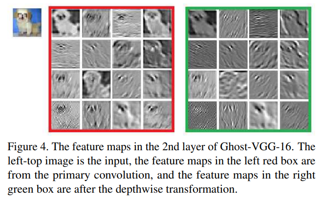
Further, the authors visualize the difference observed in the feature maps generated by standard convolutional layers and ghost convolutional layers for the 2nd layer in a VGG-16 Ghost Network, as shown below. Ghost convolution reduces the spatial redundancy and creates a unique set of feature maps with richer representations.
GhostNet Shortcomings
While the paper provides really strong results, there are some heavy shortcomings to this approach:
- The GhostNet results are compared with other standard architectures, however they don't follow the exact same training settings and tune their initial learning rate and batch size, thus resulting in an unfair comparison.
- Although using depthwise convolution seems reasonable and efficient, it isn't that straightforward. Depthwise convolutions are notorious for being non-optimized and bad on hardware. Further details are pointed out in this article. Thus, it doesn't result in the real speed improvements that one would expect with such compression techniques. This has been pointed out by several users in this issue in the official repository, to which the authors replied:
Ghost module is more suitable for ARM/CPU, and not friendly for GPU due to the Depthwise Conv.
3. Since the Ghost Module is a combination of intrinsic and depthwise convolutions, this approach can't be used t0 compress natural depthwise convolution-based models (like MobileNet v2) where using a Ghost Module in place of the depthwise convolutions results in a huge parameter and FLOPs increment, thus rendering it useless.
4. Due to decomposing a singular function into a series of functions, the resulting intermediate tensors created cause an increase in memory. This issue was also raised by users in their repository, to which the authors replied:
The run-time GPU memory may increase because Ghost module need to cache the primary feature maps and ghost feature maps and then concat them.
Although these shortcomings might seem like a deal-breaker, it's up-to the users to judge the impact of ghost modules in neural networks by giving it a try themselves.
Thanks for reading.