Intuitive Introduction to Neural Machine Translation with Bahdanau and Luong Attention

Introduction

Neural machine translation seeks to build and train a single, massive neural network that reads a sentence and provides an accurate translation, in contrast to the conventional phrase-based translation system, which consists of many tiny sub-components tweaked independently.

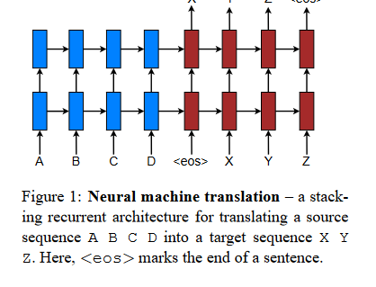
In massive translation projects, such as those from English to French(Luong et al., 2015) or English to German(Jean et al., 2015), neural machine translation (NMT) has shown state-of-the-art capabilities. NMT is attractive because it may be conceptualized with little to no prior domain expertise. The model by Luong et al. (2015) reads through all the source words until the end-of-sentence symbol<eos>is reached. As seen below, it then starts emitting the target words one at a time.

The majority of the neural machine translation models that have been proposed either belong to a family of encoder–decoders, which have an encoder and a decoder dedicated to each language, or involve applying a language-specific encoder to each sentence and then comparing the outputs of those encoders. An encoder neural network is responsible for reading a source sentence and encoding it into a vector with a specified length.

After that, a decoder will provide a translation based on the encoded vector.
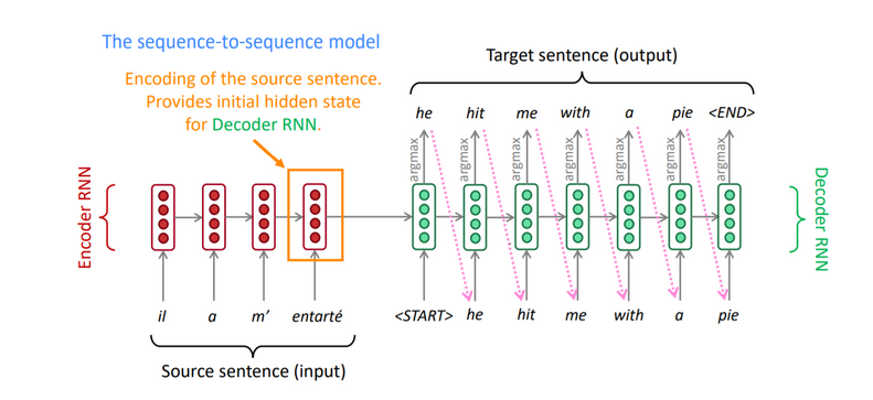
When given a source phrase, the whole encoder-decoder system, which includes both the encoder and the decoder for a particular language pair, is jointly trained to maximize the probability of producing an accurate translation. The example below shows one such implementation of NMT using an RNN-based encoder-decoder architecture.

Issue and solution

One possible drawback of the encoder-decoder method is that it requires the neural network to compress the complete source information into a vector of fixed length, and it might hinder the neural network's ability to process lengthy sentences, particularly ones much longer than those used for training.
The researchers demonstrate that the performance of a simple encoder-decoder quickly degrades with increasing input sentence length.

To solve this issue, they present a new kind of encoder-decoder model that simultaneously learns to align and translate. The suggested model (soft-)searches for a collection of points in a source sentence where the most important information is concentrated before generating a word for translation. The model then predicts a target word using the context vectors connected to the positions of the sources and all the previously generated target words.

The most important distinguishing feature of this approach from the basic encoder–decoder is that it does not attempt to encode a whole input sentence into a single fixed-length vector. Instead, it encodes the input sentence into a sequence of vectors and chooses a subset of these vectors adaptively while decoding the translation. This frees a neural translation model from having to squash all the information of a source sentence, regardless of its length, into a fixed-length vector.

In this study, the authors demonstrate that the suggested methodology of jointly learning to align and translate significantly improves translation performance compared to the standard encoder-decoder method. We can see the enhancement most clearly with longer sentences, but it works for sentences of any lengths.

Background: Neural Machine Translation

From a probabilistic point of view, translation is the same as finding the target sentence y that maximizes the conditional probability of y given the source sentence x.

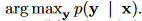
In neural machine translation, experts use a parallel training corpus to maximize the conditional probability of sentence pairings. After a translation model learns the conditional distribution for a particular source sentence, it may generate a translation by searching the sentence that maximizes the conditional probability.

The first part of this neural machine translation method encodes the source sentence x and the second part decodes it to the desired target sentence y.
For instance, a source sentence of varying length was encoded into a vector of fixed length, and the vector was then decoded into a target sentence of varying length using two recurrent neural networks (RNN). Though still in its infancy, neural machine translation has shown some impressive early successes.

On the English-to-French translation problem, it has been reported that a neural machine translation system based on RNNs with long short-term memory (LSTM) units achieves near the state-of-the-art performance of the traditional phrase-based machine translation system.

RNN Encoder–Decoder

In this paper, the authors provide a high-level overview of the RNN Encoder-Decoder foundation upon which they build their innovative architecture for learning to align and translate in tandem.

In the Encoder-Decoder framework, an encoder reads the input sentence, a sequence of vectors x, into a vector c. The most common approach is to use an RNN such that:

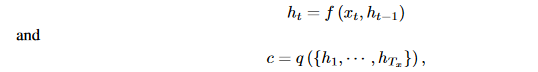
• ht is a hidden state at time t.
• c is a vector generated from the sequence of the hidden states.
• f and q are some nonlinear functions.

It is common practice to train the decoder to predict the next word yt′ using the context vector c and all the previously predicted words {y1,· · ·, yt′−1}.
Put differently, the decoder separates the joint probability into the ordered conditionals and uses those components to define a probability over the translation y.

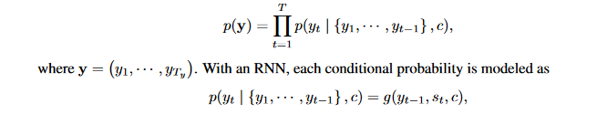
Where g is a nonlinear, potentially multi-layered function that outputs the probability of yt, and st is the hidden state of the RNN.

Decoder: General Description

In a new model architecture, the authors define each conditional probability

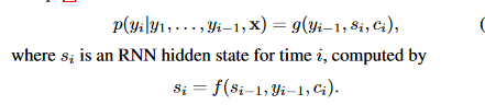
For each target word yi, the probability here is conditioned on a distinct context vector ci, in contrast to the current encoder-decoder strategy.

The context vector ci is determined by a sequence of annotations to which an encoder maps the input sentence. Each annotation hi provides information on the whole input sequence, with a significant emphasis on the parts surrounding the i-th word. The context vector ci is computed as a weighted sum of these annotations hi.

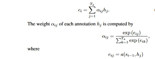
where eij is an alignment model which scores how well the inputs around position j and the output located at the position i match. The score is determined using the RNN hidden state si-1, in conjunction with the j-th annotation hj of the input sentence.

The alignment model is parameterized as a feedforward neural network and trained along with the rest of the proposed system. It's essential to keep in mind that, in contrast to conventional machine translation, alignment is not treated as a latent variable. The alignment model directly computes a soft alignment that may be backpropagated by using the cost function's gradient.This gradient can be used to train the alignment and the full translation models jointly.

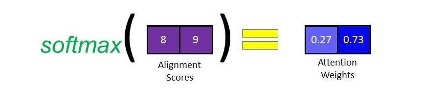
It is worth noting that we use a softmax activation function on the alignment scores to get the attention weights. To express the relative importance of each input sequence, the softmax activation function will return a set of probabilities whose sum is 1. The input sequence's importance in predicting the target word increases as its attention weight increases.

By letting the decoder have an attention mechanism, we relieve the encoder from the burden of having to encode all information in the source sentence into a fixed-length vector. With this new approach, the information can be spread throughout the sequence of annotations, which can be selectively retrieved by the decoder accordingly.

Encoder: Bidirectional RNN for annotating sequences

Assuming an input sequence x, a typical RNN will process it from the first symbol x1 through to the final symbol. We'd want each word's annotation in the proposed system to serve as a synopsis of the preceding words and the ones that will come after them. Consequently, the authors suggest using a bidirectional RNN, which has lately been used with great success in the field of voice recognition.

A BiRNN is made up of forward and backward RNNs. The forward reads the ordered input sequence and calculates a sequence of forward hidden states. The backward reads the sequence in reverse order, producing a sequence of backward hidden states.

Bahdanau Attention Process

Bahdanau's paper lays out the complete procedure for using attention in chronological order, and it goes as follows:

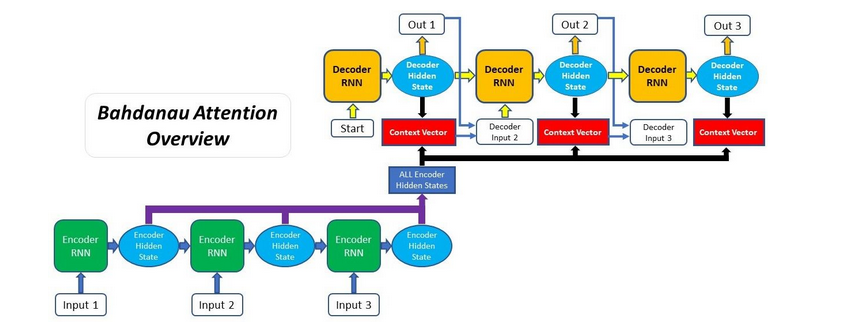
1. Generating the Encoder's Hidden States

The encoder generates hidden states for each element in the input sequence. In the first step, we'll encode the input sequence using an RNN or one of its variations (such an LSTM or GRU).
Each input sequence will generate a hidden state/output after being processed by the encoder RNN. All the encoder's hidden states will be carried on to the following time step, rather than the final hidden state.

class EncoderLSTM(nn.Module):
  def __init__(self, input_size, hidden_size, n_layers=1, drop_prob=0):
    super(EncoderLSTM, self).__init__()
    self.hidden_size = hidden_size
    self.n_layers = n_layers

    self.embedding = nn.Embedding(input_size, hidden_size)
    self.lstm = nn.LSTM(hidden_size, hidden_size, n_layers, dropout=drop_prob, batch_first=True)

  def forward(self, inputs, hidden):
    # Embed input words
    embedded = self.embedding(inputs)
    # Pass the embedded word vectors into LSTM and return all outputs
    output, hidden = self.lstm(embedded, hidden)
    return output, hidden

  def init_hidden(self, batch_size=1):
    return (torch.zeros(self.n_layers, batch_size, self.hidden_size, device=device),
            torch.zeros(self.n_layers, batch_size, self.hidden_size, device=device))

Assuming this is a linguistic task, the preceding code embeds the input words as vectors before feeding them into an LSTM encoder.

2. Calculating Alignment Scores

In the next 3 phases, we'll describe what goes on within the Attention Decoder and how the Attention mechanism is used. You'll see that the BahdanauDecoderLSTM class definition includes all three of these forward function phases.

class BahdanauDecoder(nn.Module):
  def __init__(self, hidden_size, output_size, n_layers=1, drop_prob=0.1):
    super(BahdanauDecoder, self).__init__()
    self.hidden_size = hidden_size
    self.output_size = output_size
    self.n_layers = n_layers
    self.drop_prob = drop_prob

    self.embedding = nn.Embedding(self.output_size, self.hidden_size)
    
    self.fc_hidden = nn.Linear(self.hidden_size, self.hidden_size, bias=False)
    self.fc_encoder = nn.Linear(self.hidden_size, self.hidden_size, bias=False)
    self.weight = nn.Parameter(torch.FloatTensor(1, hidden_size))
    self.attn_combine = nn.Linear(self.hidden_size * 2, self.hidden_size)
    self.dropout = nn.Dropout(self.drop_prob)
    self.lstm = nn.LSTM(self.hidden_size*2, self.hidden_size, batch_first=True)
    self.classifier = nn.Linear(self.hidden_size, self.output_size)

  def forward(self, inputs, hidden, encoder_outputs):
    encoder_outputs = encoder_outputs.squeeze()
    # Embed input words
    embedded = self.embedding(inputs).view(1, -1)
    embedded = self.dropout(embedded)
    
    # Calculating Alignment Scores
    x = torch.tanh(self.fc_hidden(hidden[0])+self.fc_encoder(encoder_outputs))
    alignment_scores = x.bmm(self.weight.unsqueeze(2))  
    
    # Softmaxing alignment scores to get Attention weights
    attn_weights = F.softmax(alignment_scores.view(1,-1), dim=1)
    
    # Multiplying the Attention weights with encoder outputs to get the context vector
    context_vector = torch.bmm(attn_weights.unsqueeze(0),
                             encoder_outputs.unsqueeze(0))
    
    # Concatenating context vector with embedded input word
    output = torch.cat((embedded, context_vector[0]), 1).unsqueeze(0)
    # Passing the concatenated vector as input to the LSTM cell
    output, hidden = self.lstm(output, hidden)
    # Passing the LSTM output through a Linear layer acting as a classifier
    output = F.log_softmax(self.classifier(output[0]), dim=1)
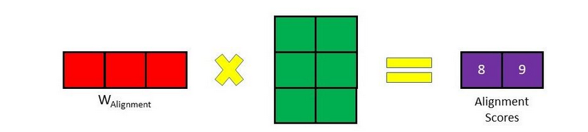
    return output, hidden, attn_weights

Once we have collected all of the outputs from the encoder, we can start utilizing the decoder to create new outputs. The decoder's alignment score for each encoder output relative to the current decoder input and hidden state must be calculated at each time step. Essentially, the Attention mechanism boils down to the alignment score, which specifies how much weight the decoder will give to each encoder output when generating the following output. Using the encoder outputs and the hidden state generated by the decoder in the preceding time step, we can get the alignment scores for Bahdanau Attention:

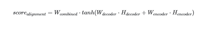
The decoder hidden state and encoder outputs will be routed via their own Linear layer, each with its own trainable weights.

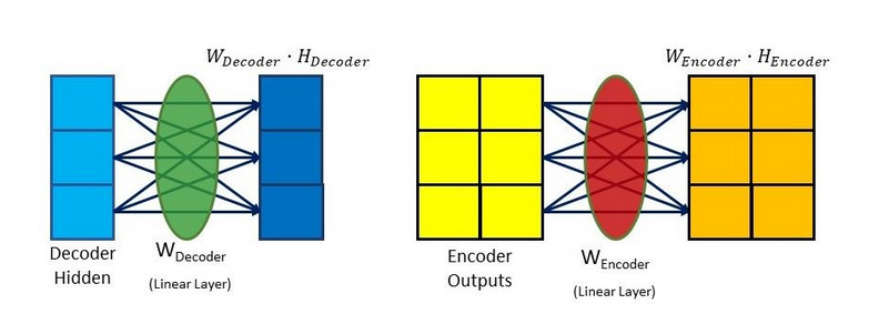
Here, we see that the hidden size is 3, and there are 2 encoder outputs. Next, they'll be combined, and then run via a tanh activation function. In this situation, the decoder's hidden state is appended to each encoder's output.

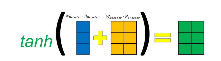
Finally, a score is assigned to each encoder output by multiplying the resulting vector by a trainable vector to get an alignment score vector.

3. Softmaxing the Alignment Scores

To determine the attention weights, we must first generate the alignment scores vector (as shown in the previous step) and then run a softmax on it. Each value in the vector, reflecting the relative importance of the various inputs at the current time step, will be between 0 and 1 as a result of the application of the softmax function.

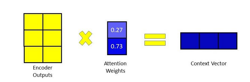
4. Calculating the Context Vector

Assuming we have already computed the attention weights, we can generate the context vector by multiplying the attention weights by the encoder outputs, element by element. The softmax function in the preceding stage enhances the impact and influence of a particular input element on the decoder output if its score is closer to 1 and diminishes its effect and influence if the score is closer to 0.

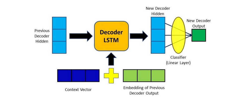
5. Decoding the Output

The output of the decoder will be added to our newly created context vector.
After that, it's sent into the decoder RNN cell to generate a new hidden state, and the process starts again from step 2. By feeding the updated hidden state into a Linear layer—a classifier that calculates probability scores for the next predicted word—we can retrieve the final output for the time step.

Luong Attention Mechanism

Multiplicative attention is another name for Luong's attention.
Simple matrix multiplications reduces the states of the encoder and the decoder into attention scores. Being speedier and taking up less space result from the matrix multiplication used. Luong proposed two types of attention mechanisms based on where the focus is put in the source sequence.

• Global attention, which focuses on all source positions.
• Local attention is focused solely on a tiny portion of the source positions per target word.

Global Attention

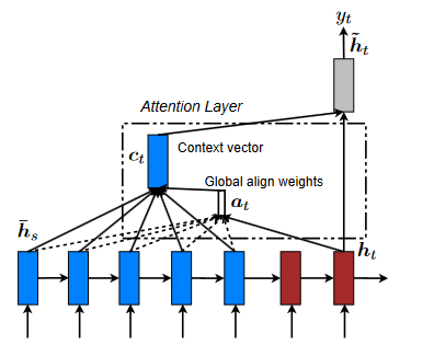
A global attentional model aims to derive the context vector ct by taking into account all the encoder's hidden states. In this model, the current target hidden state ht is compared to each source hidden state hs, yielding a variable-length alignment vector at whose size is equal to the number of time steps on the source side.

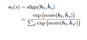
Here, score is referred as a content-based function for which we consider three different alternatives:

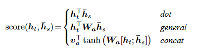
The first possibility, dot, is equivalent to multiplying the encoder's hidden state, hs, by the decoder's hidden state, ht. The second type, known as general, is similar to the dot function but also incorporates a weight matrix into the formula. As with Bahdanau Attention's calculation of alignment scores, the last function involves adding the decoder's hidden state to the encoder's hidden sate.

The difference is that the decoder hidden state and encoder hidden state are mixed together before being sent via a Linear layer. After passing through the Linear layer, the output will be subjected to a tanh activation function before being multiplied by a weight matrix to get the alignment score.

Instead of using separate weight matrices for the decoder hidden state and the encoder hidden state, like in Bahdanau Attention, they will share a single one instead.

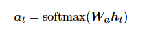
The researchers employ a location-based function in which the alignment scores are derived purely from the target hidden state ht.

The context vector ct is the weighted average of all the source hidden states, and it is produced using the alignment vector as a weight. Since the Global attention model considers the whole source sentence to make predictions about the target words, it may be challenging and time-consuming to translate lengthy sentences.

Luong Attention process

1. Producing the Encoder Hidden States

The encoder generates a hidden state for each input sequence element, much as Bahdanau Attention.

2. Decoder RNN

The RNN is used earlier in the decoding process in Luong Attention than it is in Bahdanau Attention. The RNN will utilize the previous hidden state and the word embedding of the last output to generate a new hidden state for use in the next time step.

class LuongDecoder(nn.Module):
  def __init__(self, hidden_size, output_size, attention, n_layers=1, drop_prob=0.1):
    super(LuongDecoder, self).__init__()
    self.hidden_size = hidden_size
    self.output_size = output_size
    self.n_layers = n_layers
    self.drop_prob = drop_prob
    
    # The Attention Mechanism is defined in a separate class
    self.attention = attention
    
    self.embedding = nn.Embedding(self.output_size, self.hidden_size)
    self.dropout = nn.Dropout(self.drop_prob)
    self.lstm = nn.LSTM(self.hidden_size, self.hidden_size)
    self.classifier = nn.Linear(self.hidden_size*2, self.output_size)
    
  def forward(self, inputs, hidden, encoder_outputs):
    # Embed input words
    embedded = self.embedding(inputs).view(1,1,-1)
    embedded = self.dropout(embedded)
    
    # Passing previous output word (embedded) and hidden state into LSTM cell
    lstm_out, hidden = self.lstm(embedded, hidden)
    
    # Calculating Alignment Scores - see Attention class for the forward pass function
    alignment_scores = self.attention(lstm_out,encoder_outputs)
    # Softmaxing alignment scores to obtain Attention weights
    attn_weights = F.softmax(alignment_scores.view(1,-1), dim=1)
    
    # Multiplying Attention weights with encoder outputs to get context vector
    context_vector = torch.bmm(attn_weights.unsqueeze(0),encoder_outputs)
    
    # Concatenating output from LSTM with context vector
    output = torch.cat((lstm_out, context_vector),-1)
    # Pass concatenated vector through Linear layer acting as a Classifier
    output = F.log_softmax(self.classifier(output[0]), dim=1)
    return output, hidden, attn_weights
  
class Attention(nn.Module):
  def __init__(self, hidden_size, method="dot"):
    super(Attention, self).__init__()
    self.method = method
    self.hidden_size = hidden_size
    
    # Defining the layers/weights required depending on alignment scoring method
    if method == "general":
      self.fc = nn.Linear(hidden_size, hidden_size, bias=False)
      
    elif method == "concat":
      self.fc = nn.Linear(hidden_size, hidden_size, bias=False)
      self.weight = nn.Parameter(torch.FloatTensor(1, hidden_size))
  
  def forward(self, decoder_hidden, encoder_outputs):
    if self.method == "dot":
      # For the dot scoring method, no weights or linear layers are involved
      return encoder_outputs.bmm(decoder_hidden.view(1,-1,1)).squeeze(-1)
    
    elif self.method == "general":
      # For general scoring, decoder hidden state is passed through linear layers to introduce a weight matrix
      out = self.fc(decoder_hidden)
      return encoder_outputs.bmm(out.view(1,-1,1)).squeeze(-1)
    
    elif self.method == "concat":
      # For concat scoring, decoder hidden state and encoder outputs are concatenated first
      out = torch.tanh(self.fc(decoder_hidden+encoder_outputs))
      return out.bmm(self.weight.unsqueeze(-1)).squeeze(-1)

Let me walk you through a quick illustration of the dot scoring function in case you're lost. I think you'll find this explanation.

3. Calculating Alignment Scores

The alignment score function can be specified in one of three methods in Luong Attention: dot, general, or concat. Alignment scores are computed by these scoring functions using encoder outputs and the decoder hidden state generated in the previous step.

4. Softmaxing the Alignment Scores

Alignment scores are softmaxed similarly to Bahdanau Attention, yielding weights between 0 and 1.

5. Calculating the Context Vector

This operation is identical to the one used in Bahdanau Attention, where the attention weights are multiplied by the encoder outputs.

6. Producing the Final Output

At finally, the decoder hidden state formed in Step 2 is appended to the resulting context vector. Next, we feed this combined vector into a Linear layer, which serves as a classifier, to calculate the probability scores for the next candidate word.

Local Attention

• The disadvantage of global attention is that it is time-consuming and perhaps unfeasible to translate longer sequences since it must pay attention to all words on the source side for each target word. To remedy this shortcoming, the researchers propose a local attentional method that selects a subset of the source positions per target word.
• With the image caption generation job in mind, this model is influenced by the compromise between soft and hard attentional models proposed by Xu et al. (2015). Their technique employs a global attention strategy in which weights are distributed "softly" over all input image areas. The hard attention method chooses a single area of the image to focus on at a time.
• The hard attention model is non-differentiable and requires more involved training methods like variance reduction or reinforcement learning while inexpensive at inference time.
• Local attention is very selective, allowing us to focus on a small window of context. One benefit of this method is that it is simpler to train than the hard attention method while also avoiding the costly computation required by the soft attention method.
• In concrete details, the model first generates an aligned position pt for each target word at time t. The context vector ct is then derived as a weighted average over the set of source hidden states within the window [pt−D, pt+D]; D is empirically selected.

Monotonic and Predictive Alignment

The researchers consider two variants of the model as below:

• Monotonic alignment (local-m) – they simply set pt = t assuming that source and target sequences are roughly monotonically aligned.
• Predictive alignment (local-p) – instead of assuming monotonic alignments, the model predicts an aligned position as follows:

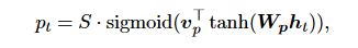
Wp and vp are the model parameters which will be learned to predict positions. S is the source sentence length.

Comparison to Bahdanau Attention

Although there are some similarities between the global attention method and the model presented by Bahdanau et al., there are also significant differences that are indicative of the simplification and generalization that have taken place.

• The encoder and decoder both rely on the same simple technique of using hidden states at the top LSTM layers.
• Concatenation of the forward and backward source hidden states in the bi-directional encoder and target hidden states in their non-stacking uni-directional decoder.
• When computing the alignment vector, the Luong attention mechanism uses the current decoder's hidden state, whereas the Bahdanau attention mechanism uses the previous hidden state.
• Bahdanau solely employs the concat score alignment model, whereas Luong uses the dot, general, and concat score alignment models.

Conclusion

The standard method for neural machine translation, known as an encoder-decoder technique, involves encoding an entire input sentence into a vector of a specified length, then decoding the vector to provide a translation.
Based on a previous empirical investigation, the authors hypothesized that using a fixed-length context vector creates issues when translating extended sentences.
To solve this problem, they developed an innovative architecture.

They went beyond the standard encoder-decoder setup by allowing each target word to be generated after a model (soft-)searched for a set of input words or their annotations computed by an encoder. This relieves the model of the burden of encoding the whole source sentence into a fixed-length vector and allows it to zero in on information that is directly pertinent to the production of the next target word. It dramatically improves the neural machine translation system's potential to translate lengthy sentences accurately.

In addition, we provide two easy-to-implement attention mechanisms for neural machine translation: a global method that considers all source positions and a local approach that focuses on a subset of source positions at a time.

References

Attention Mechanism: https://blog.floydhub.com/attention-mechanism/
Effective Approaches to Attention-based Neural Machine Translation: https://arxiv.org/pdf/1508.04025.pdf
Attention: Sequence 2 Sequence model with Attention Mechanism: https://towardsdatascience.com/sequence-2-sequence-model-with-attention-mechanism-9e9ca2a613a
Neural Machine Translation By Jointly Learning to Align And Translate: https://arxiv.org/pdf/1409.0473.pdf