Deep learning models are known to be ‘black boxes’ because they contain a degree of randomness which they use to predict ‘magical’ results that make sense to us humans. Image generation models are deep learning models that are trained on thousands if not millions of images today and it is impossible to detail all the information they learn from the training data which is then used to generate photorealistic images. What we do know for sure is that input images from the training data are encoded into an intermediate form which the model thoroughly examines to determine the most important features of the input data. The hyperspace in which these intermediate representations (vectors) are examined is known as the latent space.
In this article, I’ll review some features of the general latent space and focus on a specific latent space known as the Style Space. Style Space is the hyperspace of the channel-wise style parameters, $S$, which can be analyzed to determine which style codes correspond to specific attributes.
How Have Previous Models Used The Latent Space?
Generative Adversarial Networks (GANs) encode input data into latent vectors using learned encoder MultiLayer Perceptrons. Once the data has been encoded, it can then be decoded and upsampled into a reasonable image using learned de-convolutional layers.
StyleGAN, arguably the most iconic GAN, is best known for its generator model which converts latent vectors into an intermediate latent space using a learned mapping network. The reason for the intermediate latent space is to enforce disentanglement. The generator draws latent vectors from this intermediate space and then applies transformations on them to encode style either by normalizing feature maps or injecting noise.
After these operations, the generator decodes and upsamples these latent vectors encoded with the style to generate new artificial images bearing the visual representation of the style. Although this article is not meant to focus solely on StyleGAN, it helps to understand how the model works because its architecture paved the way for some expansive research on image representation in the latent space.
What is ‘Disentanglement’? What Does It Mean To Be ‘Entangled’?
Image training data is transformed from its high-dimensional tensor structure into latent vectors which represent the most descriptive features of the data. These features are often referred to as the ‘high variance’ features. With this new representation of the data, there is a possibility that the encoding of one attribute, $a$, holds information about a different attribute, $b$. Therefore image generation models that alter attribute, $a$, will inadvertently alter attribute $b$. $a$ and $b$ are referred to as entangled representations and the hyperspace that these vector representations exist in is an entangled latent space. Representations (vectors) representations are said to be disentangled if each latent dimension controls a single visual attribute of the image. If each latent dimension controls a single visual attribute and each attribute is controlled by a single latent dimension, then the representations are referred to as complete representations.
What Does StyleGAN Teach Us About The Latent Space?
Most GANs are trained to invert the training data into latent space representations by compressing the data into lower-dimension representations. The latent space is a hyperspace created by training an encoder to map input images to their appropriate representations in the latent space. The encoder is trained using an auto-encoder architecture; the encoder compresses the input image into a low-dimensional vector and the decoder upsamples the vector into a full high-dimensional image. The loss function compares the generated image and the input image and adjusts the parameters of the encoder and decoder accordingly.
The initial StyleGAN model introduced the idea of an intermediate latent space $W$ which is created by passing the latent vectors in the original latent space $Z$ through a learned mapping network. The reason for transforming the original vectors $z \in Z$ into the intermediate representations $w \in W$ is to achieve a disentangled latent space.
Manipulating an image in the latent feature space requires finding a matching latent code $w$ for it first. In StyleGAN 2 the authors discovered that a better way to improve the results is if you use a different $w$ for each layer of the generator. Extending the latent space by using a different $w$ for each layer finds a closer image to the given input image however it also enables projecting arbitrary images that should have no representation. To fix this, they concentrate on finding latent codes in the original, unextended latent space which correspond to images the generator could have produced.
In StyleGAN XL, the GAN was tasked to generate images from a large-scale multi-class dataset. In addition to encoding the image attributes within the vector representations in the latent space, the vectors also need to encode the class information of the input data. StyleGAN inherently works with a latent dimension of size 512. This degree of dimensionality is pretty high for natural image datasets (ImageNet’s dimension is ~40). A latent size code of 512 is highly redundant and makes the mapping network’s task harder at the beginning of training. To fix this, the authors reduce StyleGAN’s latent code $z$ to 64 to have stable training and lower FID values. Conditioning the model on class information is essential to control the sample class and improve overall performance. In a class-conditional StyleGAN, a one-hot encoded label is embedded into a 512-dimensional vector and concatenated with z. For the discriminator, class information is projected onto the last layer.
How Does StyleGAN Style The Images?
Once an image has been inverted into the latent space $z \in Z$ and then mapped into the intermediate latent space $w \in W$, “learned affine transformations then specialize $w$ into styles that control Adaptive Instance Normalization (AdaIN) operations after each convolution layer of the synthesis network $G$. The AdaIN operations normalize each feature map of the input data separately, thereafter the normalized vectors are scaled and biased by the corresponding style vector that is injected into the operation.” (Oanda 2023) Various style vectors encode different changes to different features of the image e.g. hairstyle style, skin tone, illumination of the image, etc. To distinguish the style vectors that affect specific image attributes, we need to turn our attention to the style space.
Is There A More Disentangled Space Than The Latent Space $W$? Yes — Style Space
The Style Space is the hyperspace of the channel-wise style parameters, $S$, and is significantly more disentangled than the other intermediate latent spaced explored by previous models. The style vectors a.k.a style codes referred to in the previous section contain various style channels that affect different local regions of an image. My understanding of the difference between style vectors and style channels can be explained by the following example, “A style vector that edits the person’s lip makeup can contain style channels that determine the boundaries of the lips in the edited generated image.” The authors who discovered the Style Space describe a method for discovering a large collection of style channels, each of which is shown to control a distinct visual attribute in a highly localized and disentangled manner. They propose a simple method for identifying style channels that control a specific attribute using a pre-trained channel classifier or a small number of example images. In addition to creating a method to classify different style channels, the authors also create a new metric “Attribute Dependency Metric” to measure the disentanglement in generated and edited images.
After the network processes the intermediate latent vector $w$, the latent code is used to modify the channel-wise activation statistics at each of the generator’s convolution layers. To modulate channel-wise means and variances, StyleGAN uses AdaIN operations described above. Some control over the generated results may be obtained by conditioning, which requires training the model with annotated data. The style-based design enables the discovery of a variety of interpretable generator controls after training the generator. However, most style-based design methods require pretrained classifiers, a large set of paired examples, or manual examination of many candidate control directions and this limits the versatility of these methods. Additionally, the individual controls discovered by these methods are typically entangled and non-local.
Proving the Validity of Style Space, $S$
The first latent space $Z$ is typically normally distributed. The random noise vectors $z \in Z$ are transformed into an intermediate latent space $W$ via a sequence of fully connected layers. $W$ space was found to better reflect the disentangled nature of the learned distribution with the inception of StyleGAN. To create the style space, each $w \in W$ is further transformed to channel-wise style parameters $s$, using a different learned affine transformation for each layer of the generator. These channel-wise parameters exist in a new distribution known as the $\text{Style Space or S}$.
After the introduction of the intermediate space, $W$, other researchers introduced another latent space $W+$ because they noticed it was difficult to reliably embed images into the $Z \text{ and }W$ spaces. $W +$ is a concatenation of 18 different 512-dimensional w vectors, one for each layer of the StyleGAN architecture that can receive input via AdaIN. The $Z$ space has 512 dimensions, the $W$ space has 512 dimensions, the $W+$ space has 9216 dimensions, and the $S$ space has 9088 dimensions. Within the $S$ space, 6048 dimensions are applied to feature maps, and 3040 dimensions are applied to tRGB blocks. The goal of this project is to determine which of these latent spaces offers the most disentangled representation based on the disentanglement, completeness, and informativeness (DCI) metrics.
Disentanglement is the measurement of the degree to which each latent dimension captures at most one attribute. Completeness is the measure of the degree to which each attribute is controlled by at most one latent dimension. Informativeness is the measure of the classification accuracy of the attributes given the latent representation.
To compare the DCI of the 3 different latent spaces, they trained 40 binary attribute classifiers based on the 40 CelebA attributes but end up basing their experiments on about ~30 of the best-represented attributes. The next step was to randomly sample 500K latent vectors $z \in Z$ and compute their corresponding $w$ and $s$ vectors, as well as the images these vectors generate. Thereafter, they annotate each image by each of the ~30 classifiers and record the logit rather than the binary outcome. The higher the logit value, the higher the degree of DCI of the hyperspace for each attribute each classifier is trained on. The informativeness of $W$ and $S$ is high and comparable, $S$ scores much higher in terms of disentanglement and completeness.
There are two main questions that the Style Space tries to answer:
- What style channels control the visual appearance of local semantic regions? This question can take the form, “What style channel(s) control a specific region of the image even if the region cannot be conventionally labeled as a known class e.g. nose?”
- What style channels control specific attributes specified by a set of positive examples? This question can take the form, “What style channel(s) controls the generation of images of a human with red hair, given a few images of people with red hair?”
Determining the Channels that Control Specific Local Semantic Regions
After they proved that Style Space, $S$, was the best suited to represent styles in the latent space, the authors proposed a method of detecting the $S$ channels that control the visual appearance of local semantic regions. To do this, they examine the gradient maps of generated images w.r.t different channels, measure the overlap with specific semantic regions, and then with this information, they can identify those changes that are consistently active in each region.
How do they get the gradient map?
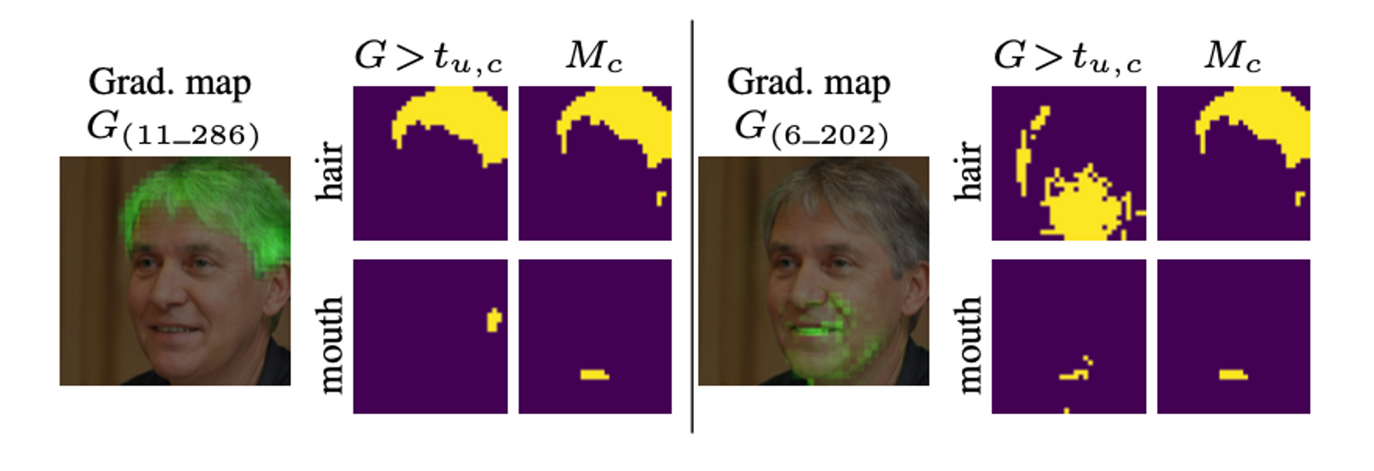
For each image generated with style code $s \in S$, apply back-propagation to compute the gradient map of the image w.r.t each channel of $s$. The gradient map helps us identify which region of the image changed when the style channel $s$ was applied and then highlights those pixels. For implementation purposes, it is important to note that the gradient maps are computed at a reduced spatial resolution $r \times r$ to save computation.
A pretrained image segmentation network is used to obtain the semantic map $M^s$ of the generated image ($M^s$ is also resized to $r \times r$). For each semantic category $c$ determined by the pre-trained model (e.g. hair) and each channel $u$ that we are evaluating, we measure the overlap between the semantic region $M_c^s$ and the gradient map $G_u^s$. The goal here is to identify distinct semantic attributes in a generated image, determine the regions that have changed as a result of a style channel $u$ , and then find the overlap between these regions and the segmented attribute regions. To ensure consistency across a variety of images, they sample 1K different style codes and compute for each code $s$ and each channel $u$ the semantic category with the highest overlap. The goal is to detect channels for which the highest overlap category is the same for the majority of the sampled images.
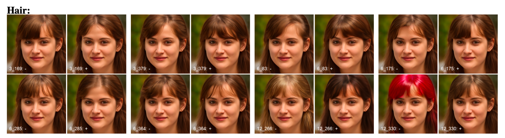
In the image above, style channels that affect portions of the hair region have been determined and are represented by the number on the lower left part of the image. For every channel $x$, there is a pair of images with the channel values $+x, -x$. The difference between the images produces by the channels $+x, -x$ shows the specific region that channel $x$ has altered.
Detecting the Channels that Control Attributes Specified by Positive Examples
To determine the channels that control specific attributes, we need to collect and compare a few positive and negative image samples where the attribute has been changed. The authors of the Style Space argue that we can make this inference using only 30 samples. Differences between the style vectors of the positive examples and the mean vector of the entire generated distribution reveal which channels are the most relevant for the target attribute. They got a set of positive images — images whose visual attributes matched the text definition — and attempted to determine the style channels that led to their styling. They got latent style vectors of the positive images and compared them to the style latent vectors of the entire dataset to confirm that these vectors are unique to the target style. We know from previous paragraphs that we can get the style channel vector by applying affine transformations to the intermediate latent vector $w$. Once we generate the style channel vector we determine its relevance to the desired attribute using the ratio $\theta_u$
How do they determine the channels relevant to a specific attribute?
The first step is getting a set of pretrained classifiers to identify the top 1K positive image examples for each of the selected attributes. For each attribute, they rank all the style channels predicted for that attribute by their relevance using the ‘relevance ratio $\theta_u$’.
In the research paper, the authors manually examined the top 30 channels to verify that they indeed control the target attribute. They determine that 16 CelebA attributes may be controlled by at least one style channel. For well-distinguished visual attributes (gender, black hair etc.) the method was only able to find one controlling attribute. The more specific the attribute, the fewer channels are needed to control it.
Because most of the detected attribute-specific control channels were highly ranked by our proposed importance score $\theta_u$. This suggests that a small number of $+ve$ examples provided by a user might be sufficient for identifying such channels. The authors note that using only 30 positive samples you can identify the channels required to create the given style changes. Increasing the number of $+ve$ examples and only considering locally-active channels in areas related to the target attribute improves detection accuracy.
Summary
The work on Style Space established a way for us to understand and identify style channels that control both local semantic regions and specific attributes defined by positive samples. The benefit of distinguishing between style channels that affect specific local regions is that, the researcher doesn’t need to have a specific attribute in mind. It’s an open-ended mapping that allows the researcher to focus on regions of interest that are not limited by conventional labels of face regions e.g nose, lips, and eye. The gradient map can spread across multiple conventional regions or cluster around a small portion of a conventional region. Having an open-ended mapping allows the researcher to identify style changes without bias e.g the hair editing channel (above) that changes the sparsity of hair on someone’s bangs. The method that uses positive attribute examples allows the researcher to identify the style channels that control specific attributes without the need for a gradient map or any image segmentation technique. This method would be really helpful if you had a few positive examples of a rare attribute and you wanted to find the corresponding style channels. Once you find the style vectors and channels that control the given attribute, you could intentionally generate more images with the rare attribute to augment some sort of training data. There is a lot more ground to cover in terms of exploring and exploiting the latent space but this is a comprehensive review of the tools we can gain from focusing on the Style Space $S$.
Citations:
- Karras, Tero, Samuli Laine, and Timo Aila. "A style-based generator architecture for generative adversarial networks." Proceedings of the IEEE/CVF conference on computer vision and pattern recognition. 2019.
- Karras, Tero, et al. "Analyzing and improving the image quality of stylegan." Proceedings of the IEEE/CVF conference on computer vision and pattern recognition. 2020.
- Karras, Tero, et al. "Alias-free generative adversarial networks." Advances in Neural Information Processing Systems 34 (2021): 852-863.
- Abdal, Rameen, Yipeng Qin, and Peter Wonka. "Image2stylegan: How to embed images into the stylegan latent space?." Proceedings of the IEEE/CVF International Conference on Computer Vision. 2019.
- Wu, Zongze, Dani Lischinski, and Eli Shechtman. "Stylespace analysis: Disentangled controls for stylegan image generation." Proceedings of the IEEE/CVF Conference on Computer Vision and Pattern Recognition. 2021.