MDP: Text-guided Image Editing by Manipulating Diffusion Path

Text-based image generation techniques have prevailed recently. Specifically, diffusion models have shown tremendous success in a different types of text-to-image works. Stable diffusion can generate photorealistic images by giving it text prompts. After the success of image synthesis models, the amount of focus grew on image editing research. This research focuses on editing images (either real images or images synthesized by any model) by providing text prompts on what to edit in the image. There have been many models that came out as part of image editing research but almost all of them focus on training another model to edit the image. Even if the diffusion models have the ability to synthesize images, these models train another model in order to edit the images.

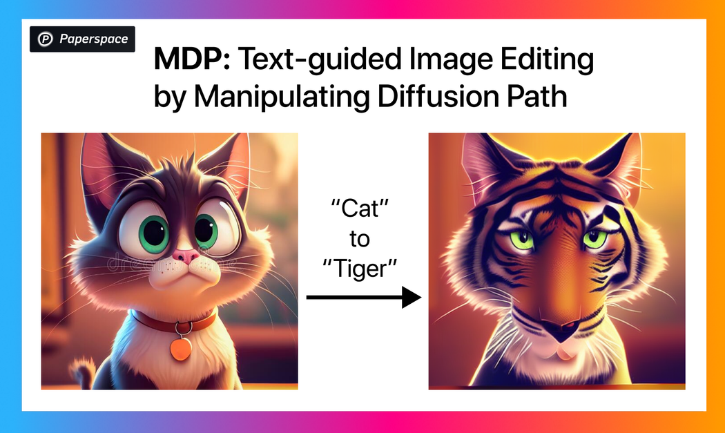
Recent research on Text-guided Image Editing by Manipulating Diffusion Path focuses on editing images based on the text prompt without training another model. It utilizes the inherent capabilities of the diffusion model to synthesize images. The image synthesis process path can be altered based on the edit text prompt and it will generate the edited image. Since this process solely relies on the quality of the underlying diffusion model, it doesn't require any additional training.

Basics of Diffusion Models

The objective behind the diffusion model is really simple. The objective is to learn to synthesize photorealistic images. The diffusion model consists of two processes: the forward diffusion process and the reverse diffusion process. Both of these diffusion processes follow the traditional Markov Chain principle.

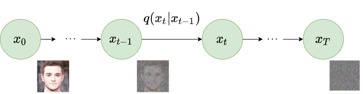
As part of the forward diffusion process, the noise is added to the image so that it is directly recognizable. To do that it first samples a random image from the dataset, say $x_0$. Now, the diffusion process iterates for total $T$ timesteps. At each time step $t$ ($0 < t \le T$), gaussian noise is added to the image at the previous timestep to generate a new image. i.e. $q(x_t \lvert x_{t-1})$. The following image explains the forward diffusion process.

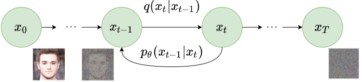
As part of the reverse diffusion process, the noisy image generated as part of the forward diffusion process is taken as input. The diffusion process again iterates for total $T$ timesteps. At each timestep $t$ ($0 < t \le T$), the model tries to remove the noise from the image to produce a new image. i.e. $p_{\theta}(x_{t-1} \lvert x_t)$. The following image explains the reverse diffusion process.

By recreating the real image from the noisy image, the model learns to synthesize the image. The loss function only compares the noise added and noise removed at corresponding timesteps in each forward and reverse diffusion process. We would recommend understanding the mathematics of the diffusion models to understand the rest of the content of this blog. We highly recommend reading this AISummer article to develop a mathematical understanding of diffusion models.

Additionally, CLIP (Contrastive-Image-Language-Pretraining) can be used so that the relevant text prompt can affect the image generation process. Thus, we can generate images based on the given text prompts.

Manipulating Diffusion Path

Research done as part of the MDP paper argues that we do not need any additional model training to edit the images using the diffusion technique. Instead, we can use the pre-trained diffusion model and we can change the diffusion path based on the edit text prompt to generate the edited image itself. By altering $q(x_t \lvert x_{t-1})$ and $p_{\theta}(x_{t-1} \lvert x_t)$ for a few timesteps based on the edit text prompt, we can synthesize the edited image. For this paper, the authors refer to text prompts as conditions. It means that we can do the image editing task by combining the layout from the input image and altering relevant things in the image based on provided condition. To edit the image based on condition, conditional embedding generated from the text prompt is used.

The editing process can be carried out in two different cases based on the provided input. The first case is that we are only given an input image $x^A$ and the conditional embedding corresponding to edit task $c^B$. Our task is to generate an edited image $x^B$ which has been generated by changing the diffusion path of $x^A$ based on condition $c^B$.

The second case is that we are given input condition embedding $c^A$ and the conditional embedding corresponding to edit task $c^B$. Our task is to first generate input image $x^A$ based on input condition embedding $c^A$, then to generate an edited image $x^B$ which has been generated by changing the diffusion path of $x^A$ based on condition $c^B$.

If we look closely, the first case described above is the subset of the second case. To unify both of these into a single framework, we would need to predict $c^A$ in the first case described above. If we can determine the conditional embedding $c^A$ from the input image $x^A$, both cases can be processed in the same way for to find the final edited image. To find conditional embedding $c^A$ from input image $x^A$, authors have used the Null Text Inversion process. This process carries out both diffusion processes and finds the embedding $c^A$. You can think of it as predicting the sentence from which the image $x^A$ can be generated. Please read the paper on Null Text Inversion for more information about it.

Now we have unified both cases, we can now modify the diffusion path to get the edited image. Let us say we selected sets of timesteps to modify in the diffusion path to get the edited image. But what should we modify? So, there are 4 factors we can modify for particular timestep $t$ ($0 < t \le T$): (1) We can modify the predicted noise $\epsilon_t$. (2) We can modify the conditional embedding $c_t$. (3) We can modify the latent image tensor $x_t$ (4) We can modify the guidance scale $\beta$ which is the difference between the predicted noise from the edited diffusion path and the original diffusion path. Based on these 4 cases, the authors describe 4 different algorithms which can be implemented to edit images. Let us take a look at them one by one and understand the mathematics behind them.

MDP-$\epsilon_t$

This case focuses on modifying only the predicted noise at timestep $t$ ($0 < t \le T$) during the reverse diffusion process. At the start of the reverse diffusion process, we will have the noisy image $x_T^A$, conditional embedding $c^A$ and conditional embedding $c^B$. We will iterate in reverse from timestep $T$ to $1$ to modify the noise. At relevant timestep $t$ ($0 < t \le T$), we will apply following modifications:

$$\epsilon_t^B = \epsilon_{\theta}(x_t^*, c^B, t)$$

$$\epsilon_t^* = (1-w_t) \epsilon_t^B + w_t \epsilon_t^*$$

$$x_{t-1}^* = DDIM(x_t^*, \epsilon_t^*, t)$$

We first predict the noise using the $\epsilon_t^B$ corresponding to the image in the current timestep and condition embedding $c^B$ using the UNet block of the diffusion model. Don't get confused by $x_t^*$ here. Initially, we start with $x_T^A$ at timestep $T$ but we refer to the intermediate image at timestep $t$ as $x_t^*$ because it is no longer only conditioned by $c^A$ but also $c^B$. The same is also applicable to $\epsilon_t^*$.

After calculating $\epsilon_t^B$, we can now calculate the $\epsilon_t^*$ as a linear combination of $\epsilon_t^B$ (conditioned by $c^B$) and $\epsilon_t^*$ (original diffusion path). Here, parameter $w_t$ can be set to constant or can be scheduled for different timesteps. Once we calculate $\epsilon_t^*$, we can apply DDIM (Denoising Diffusion Implicit Models) that generates an image for the previous timestep. This way, we can alter the diffusion path of several (or all) timesteps of the reverse diffusion process to edit the image.

MDP-$c$

This case focuses on modifying only the condition ($c$) at timestep $t$ ($0 < t \le T$) during the reverse diffusion process. At the start of the reverse diffusion process, we will have the noisy image $x_T^A$, conditional embedding $c^A$ and conditional embedding $c^B$. At each step, we will modify the combined condition embedding $c_t^*$. At relevant timestep $t$ ($0 < t \le T$), we will apply following modifications:

$$c_t^* = (1-w_t)c^B + w_tc_t^*$$

$$\epsilon_t^* = \epsilon_{\theta}(x_t^*, c_t^*, t)$$

$$x_{t-1}^* = DDIM(x_t^*, \epsilon_t^*, t)$$

We first calculate the combined embedding $c_t^*$ for timestep $t$ by taking a linear combination of $c^B$ (condition embedding for edit text prompt) and $c_t^*$ (condition embedding for original diffusion steps). Here, parameter $w_t$ can be set to constant or can be scheduled for different timesteps. In the second step, we predict $\epsilon_t^*$ using this newly calculated condition embedding $c_t^*$. The last step generates an image for the previous timestep using DDIM.

MDP-$x_t$

This case focuses on modifying only the generated image itself ($x_{t-1}$) at timestep $t$ ($0 < t \le T$) during the reverse diffusion process. At the start of the reverse diffusion process, we will have the noisy image $x_T^A$, conditional embedding $c^A$ and conditional embedding $c^B$. At each step, we will modify the generated image $x_{t-1}^*$. At relevant timestep $t$ ($0 < t \le T$), we will apply following modifications:

$$\epsilon_t^B = \epsilon_{\theta}(x_t^*, c^B, t)$$

$$x_{t-1}^* = DDIM(x_t^*, \epsilon_t^B, t)$$

$$x_{t-1}^* = (1-w_t) x_{t-1}^{*} + w_tx_{t-1}^A$$

We first predict the noise $\epsilon_t^B$ corresponding to the condition embedding $c^B$. Then, we generate the image $x_{t-1}^*$ using DDIM. At last, we take a linear combination of $x_{t-1}^{B*}$ (conditioned by $c^B$) and $x_{t-1}^A$ (original diffusion path). Here, parameter $w_t$ can be set to constant or can be scheduled for different timesteps.

MDP-$\beta$

This case focuses on modifying the guidance scale by calculating the predicted noise of both conditions and taking a linear combination of it. At the start of the reverse diffusion process, we will have the noisy image $x_T^A$, conditional embedding $c^A$ and conditional embedding $c^B$. At each step, we will modify the generated image $\epsilon_t^*$. At relevant timestep $t$ ($0 < t \le T$), we will apply following modifications:

$$\epsilon_t^A = \epsilon_{\theta}(x_t^*, c^A, t)$$

$$\epsilon_t^B = \epsilon_{\theta}(x_t^*, c^B, t)$$

$$\epsilon_t^* = (1-w_t) \epsilon_t^B + w_t \epsilon_t^A$$

$$x_{t-1}^* = DDIM(x_t^*, \epsilon_t^*, t)$$

We first predict the noise $\epsilon_t^A$ and $\epsilon_t^B$ corresponding to two condition embeddings $c^A$ and $c^B$ respectively. We then take a linear combination of those two to calculate $\epsilon_t^*$. Here, parameter $w_t$ can be set to constant or can be scheduled for different timesteps. The last step generates an image for the previous timestep using DDIM.

Model Performance & Comparisons

All of the 4 algorithms defined above are able to generate good-quality edited images that follow the edit text prompt. The results obtained by these algorithms are compared with Prompt-to-Prompt image editing model. Below results are provided in the research paper.

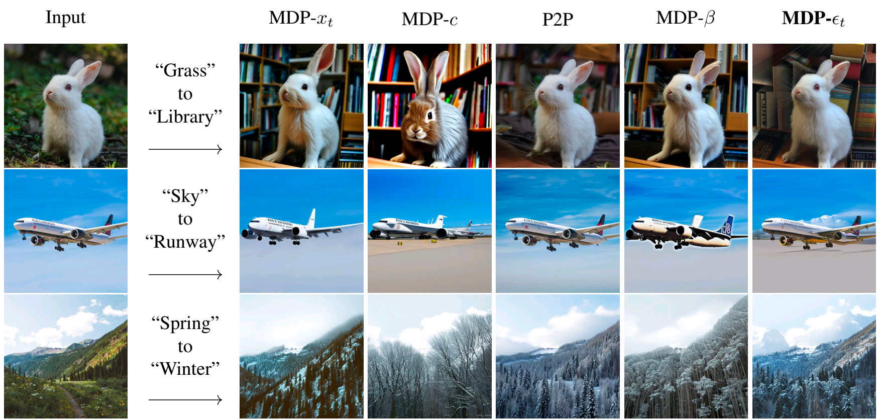
The results of these algorithms are comparable to other image editing models which employ training. The authors have argued that MDP-$\epsilon_t$ works best among all 4 algorithms in terms of local and global editing capabilities.

Try it yourself

Let us now walk through how you can try this model. The authors have open-sourced the code for only the MDP-$\epsilon_t$ algorithm. But based on the detailed descriptions, we have implemented all 4 algorithms and the Gradio demo in this GitHub Repository. The best part about MDP model is that it doesn't require any training. We just need to download the pre-trained Stable Diffusion model. But don't worry, we have taken care of this in the code. You will not need to manually fetch the checkpoints. For demo purposes, let us get this code running in a Gradient Notebook here on Paperspace. To navigate to the codebase, click on the "Run on Gradient" button above or at the top of this blog.

Setup

The file installations.sh contains all the necessary code to install required dependencies. This method doesn't require any training but the inference will be very costly and time-consuming on the CPU since diffusion models are too heavy. Thus, it is good to have CUDA support. Also, you may require different version of torch based on the version of CUDA. If you are running this on Paperspace, then the default version of CUDA is 11.6 which is compatible with this code. If you are running it somewhere else, please check your CUDA version using nvcc --version. If the version differs from ours, you may want to change versions of PyTorch libraries in the first line of installations.sh by looking at compatibility table.

To install all the dependencies, run the below command:

bash installations.sh

MDP doesn't require any training. It uses the stable diffusion model and changes the reverse diffusion path based on the edit text prompt. Thus, it enables synthesizing the edited image. We have implemented all 4 algorithms mentioned in the paper and prepared two types of Gradio demos to try out the model.

Real-Image Editing Demo

As part of this demo, you can edit any image based on the text prompt. With this, you can input any image, an edit text prompt, select the algorithm that you want to apply for editing, and modify the required algorithm parameters. The Gradio app will run the specified algorithm by taking provided inputs with specified parameters and will generate the edited image.

To run this the Gradio app, run the below command:

gradio app_real_image_editing.py

Once you run the above command, the Gradio app will generate a link that you can open to launch the app. The below video shows how you can interact with the app.

Synthetic-Image Editing Demo

As part of this demo, you can first generate an image using a text prompt and then you can edit that image using another text prompt. With this, you can input the initial text prompt to generate an image, an edit text prompt, select the algorithm that you want to apply for editing and modify the required algorithm parameters. The Gradio app will run the specified algorithm by taking provided inputs with specified parameters and will generate the edited image.

To run this Gradio app, run the below command:

gradio app_synthetic_image_editing.py

Once you run the above command, the Gradio app will generate a link that you can open to launch the app. The below video shows how you can interact with the app.

Conclusion

We can edit the image by altering the path of the reverse diffusion process in a pre-trained Stable Diffusion model. MDP utilizes this principle and enables editing an image without training any additional model. The results are comparable to other image editing models which use training procedures. In this blog, we walked through the basics of the diffusion model, the objective & architecture of the MDP model, compared the results obtained from 4 different MDP algorithm variants and discussed how to set up the environment & try out the model using the Gradio demos on Gradient Notebook.

Be sure to check out our repo and consider contributing to it!