Bring this project to life
In this tutorial, we show how to implement a music genre classifier from scratch in TensorFlow/Keras using features calculated by the Librosa library.
We will use the most popular publicly available Dataset for music genre classification : the GTZAN. This datasets contains a range of recordings reflecting different circumstances, the files were gathered between year 2000 and 2001 from a number of sources, including personal CDs, radio, and microphone recordings. Even with the fact that it's more than 2 decades old, it is still considered as the go-to Dataset when it comes to machine learning applications regarding music genre classification.
The dataset contains 10 classes, each class with a 100 of different 30 seconds audio files. The classes are: blues, classical, country, disco, hip-hop, jazz, metal, pop, reggae and rock.
In this tutorial, we will only use 3 genres (reggae, rock and classical) for simplification purposes. But, the same principles are still valid for higher numbers of genres.
Let's start by downloading and extracting the Dataset files.
Preparing the Dataset
We first will download the files from Google Drive using the gdrive package. We will then unarchive each of the files using unrar from the terminal. You can do this with the command line or using line magic.
gdown --fuzzy 'https://drive.google.com/file/d/1nZz6EHYl7M6ReCd7BUHzhuDN52mA36_q/view?usp=drivesdk'
7z e gtzan.rar -odataset_rar
unrar e dataset_rar/reggae.rar dataset/reggae/
unrar e dataset_rar/rock.rar dataset/rock/
unrar e dataset_rar/classical.rar dataset/classical/Importing python libraries
Now we'll import the needed libraries. TensorFlow will be used for model training, evaluation and prediction, Librosa for all the audio related manipulations including feature generation, Numpy for numerical handling and Matplotlib for printing the features as images.
import os
import numpy
from tensorflow import keras
import librosa
from matplotlib import pyplotAudio features
Each music genre is characterized by its own specifications: pitch, melody, chord progressions and instrumentation type. To have a reliable classification, we will use a set of features that capture the essence of these elements, giving the model a better chance to be properly trained to distinguish between genres.
In this tutorial, we'll construct four features that we will be used to create a single feature vector related to each file that our model will be trained on.
These features are:
- Mel frequency Cepstral coefficiens
- Mel spectogram
- Chroma vector
- Tonal Centroid Features
Mel Frequency Cepstral Coefficients (MFCC)
MFCCs or Mel-Frequency Cepstral Coefficients are Cepstral coefficients calculated by a discrete cosine transform applied to the power spectrum of a signal. The frequency bands of this spectrum are spaced logarithmically according to the Mel scale.
def get_mfcc(wav_file_path):
  y, sr = librosa.load(wav_file_path, offset=0, duration=30)
  mfcc = numpy.array(librosa.feature.mfcc(y=y, sr=sr))
return mfccNext, we'll plot the MFCC image of an example file, using Matplotlib:
example_file = "dataset/classical/classical.00015.wav"
mfcc = get_mfcc(example_file)
pyplot.imshow(mfcc, interpolation='nearest', aspect='auto')
pyplot.show()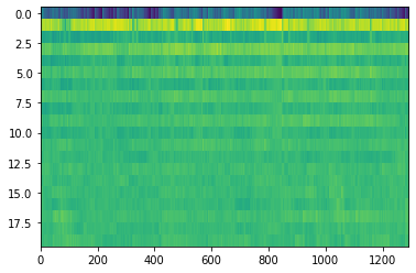
Mel Spectrogram
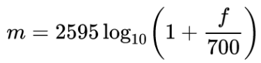
The Mel spectrogram is equal to the standard spectrogram in the Mel scale, which is a perceptual scale of pitches that listeners perceive to be equally spaced from one another. The conversion from the frequency domain in hertz to the Mel scale is done using the following formula:
def get_melspectrogram(wav_file_path):
  y, sr = librosa.load(wav_file_path, offset=0, duration=30)
  melspectrogram = numpy.array(librosa.feature.melspectrogram(y=y, sr=sr))
return melspectrogramNext, we plot the Mel spectrogram for the same audio file:
melspectrogram = get_melspectrogram(example_file)
pyplot.imshow(melspectrogram, interpolation='nearest', aspect='auto')
pyplot.show()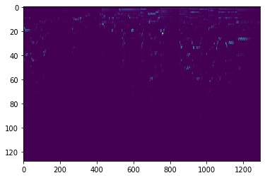
Chroma Vector
The Chroma features vector is constructed by having the full spectrum projected onto 12 bins that reflect the 12 unique semitones (or Chroma) of the musical octave: C, C#, D, D#, E , F, F#, G, G#, A, A#, B. This projection gives an intriguing and potent representation of music audio and is especially dependent on the music genre.
Since notes that are exactly one octave apart are perceived as being particularly similar in music, understanding the distribution of Chroma, even without knowing the absolute frequency (i.e., the original octave), can provide useful musical information about the audio and may even expose perceived musical similarities in the same music genre that are not visible in the original spectra.
def get_chroma_vector(wav_file_path):
  y, sr = librosa.load(wav_file_path)
  chroma = numpy.array(librosa.feature.chroma_stft(y=y, sr=sr))
return chromaThe Chroma vector for the same audio sample is then plotted next:
chroma = get_chroma_vector(example_file)
pyplot.imshow(chroma, interpolation='nearest', aspect='auto')
pyplot.show()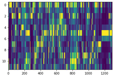
Tonal Centroid Features (Tonnetz)
This representation is calculated by projecting Chroma features onto a 6-dimensional basis representing the perfect fifth, minor third, and major third each as two-dimensional coordinates.
def get_tonnetz(wav_file_path):
  y, sr = librosa.load(wav_file_path)
  tonnetz = numpy.array(librosa.feature.tonnetz(y=y, sr=sr))
return tonnetzFor the same Chroma vector we have the following Tonnetz feature:
tntz = get_tonnetz(example_file)
pyplot.imshow(tntz , interpolation='nearest', aspect='auto')
pyplot.show()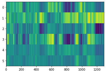
Bring this project to life
Putting the Features together
After creating the four functions for generating the features. We implement the function get_feature that will extract the envelope (min and max) and the mean of each feature along the time axis. This way, we will have a feature with constant size no matter what the length of the audio is. Next, we concatenate the four features, using Numpy, into a single 498 float array.
def get_feature(file_path):
  # Extracting MFCC feature
  mfcc = get_mfcc(file_path)
  mfcc_mean = mfcc.mean(axis=1)
  mfcc_min = mfcc.min(axis=1)
  mfcc_max = mfcc.max(axis=1)
  mfcc_feature = numpy.concatenate( (mfcc_mean, mfcc_min, mfcc_max) )

  # Extracting Mel Spectrogram feature
  melspectrogram = get_melspectrogram(file_path)
  melspectrogram_mean = melspectrogram.mean(axis=1)
  melspectrogram_min = melspectrogram.min(axis=1)
  melspectrogram_max = melspectrogram.max(axis=1)
  melspectrogram_feature = numpy.concatenate( (melspectrogram_mean, melspectrogram_min, melspectrogram_max) )

  # Extracting chroma vector feature
  chroma = get_chroma_vector(file_path)
  chroma_mean = chroma.mean(axis=1)
  chroma_min = chroma.min(axis=1)
  chroma_max = chroma.max(axis=1)
  chroma_feature = numpy.concatenate( (chroma_mean, chroma_min, chroma_max) )

  # Extracting tonnetz feature
  tntz = get_tonnetz(file_path)
  tntz_mean = tntz.mean(axis=1)
  tntz_min = tntz.min(axis=1)
  tntz_max = tntz.max(axis=1)
  tntz_feature = numpy.concatenate( (tntz_mean, tntz_min, tntz_max) )

  feature = numpy.concatenate( (chroma_feature, melspectrogram_feature, mfcc_feature, tntz_feature) )
return featureCalculating features for the full Dataset
Now, we'll use three genres to train our model on: reggae, classical and rock. For more nuances, like distinguishing between genres that have a lot of similarities, Rock and Metal for example, more features should be included.
We'll loop through each file of these three genres. And, for each one we'll construct the feature array and store it along with the respective label.
directory = 'dataset'
genres = ['reggae','classical','rock']
features = []
labels = []
for genre in genres:
    print("Calculating features for genre : " + genre)
    for file in os.listdir(directory+"/"+genre):
        file_path = directory+"/"+genre+"/"+file

        features.append(get_feature(file_path))
        label = genres.index(genre)
labels.append(label)Splitting the Dataset into training, validation and testing parts
After creating the feature and label arrays, we use Numpy to shuffle the records. Then, split the Dataset into training, validation and testing parts: 60%, 20% and 20% respectively.
permutations = numpy.random.permutation(300)
features = numpy.array(features)[permutations]
labels = numpy.array(labels)[permutations]

features_train = features[0:180]
labels_train = labels[0:180]

features_val = features[180:240]
labels_val = labels[180:240]

features_test = features[240:300]
labels_test = labels[240:300]Training the model
For this model, we will implement using Keras two regular densely connected neural network layers, with a rectified linear unit activation function "relu", and 300 hidden units for the first layer and 200 for second layer. Then, for the output layer we will also implement a densely connected layer with the probabilistic distribution activation function "softmax". Then we'll train the model using 64 epochs:
inputs = keras.Input(shape=(498), name="feature")
x = keras.layers.Dense(300, activation="relu", name="dense_1")(inputs)
x = keras.layers.Dense(200, activation="relu", name="dense_2")(x)
outputs = keras.layers.Dense(3, activation="softmax", name="predictions")(x)

model = keras.Model(inputs=inputs, outputs=outputs)

model.compile(
    # Optimizer
    optimizer=keras.optimizers.RMSprop(),
    # Loss function to minimize
    loss=keras.losses.SparseCategoricalCrossentropy(),
    # List of metrics to monitor
    metrics=[keras.metrics.SparseCategoricalAccuracy()],
)
model.fit(x=features_train.tolist(),y=labels_train.tolist(),verbose=1,validation_data=(features_val.tolist() , labels_val.tolist()), epochs=64)Model evaluation
Then, we evaluate the model:
score = model.evaluate(x=features_test.tolist(),y=labels_test.tolist(), verbose=0)
print('Accuracy : ' + str(score[1]*100) + '%')
Using this simple model and with this set of features, we can achieve an accuracy around 86%.
Accuracy : 86.33333134651184%Classification of a Youtube video
Then, we will use library youtube-dl to export a video from Youtube, that we will later classify.
pip install youtube-dlWe download the video and save it as a wave file. In this example, we use Bob Marley's "Is This Love" video clip.
youtube-dl -x --audio-format wav --output "audio_sample_full.wav" https://www.youtube.com/watch?v=69RdQFDuYPIAfter that, we install the pydub library that we'll use to crop the wav file size
pip install pydubWe crop the wav file to a 30 seconds section, from 01:00:00 tp 01:30:00. Then, save the resulting file.
from pydub import AudioSegment
t1 = 60000 #Works in milliseconds
t2 = 90000
waveFile = AudioSegment.from_file("audio_sample_full.wav")
waveFile = waveFile[t1:t2]
waveFile.export('audio_sample_30s.wav', format="wav")
Then, we use our previously trained model to classify the audio music genre of the audio.
file_path = "audio_sample_30s.wav"
feature = get_feature(file_path)
y = model.predict(feature.reshape(1,498))
ind = numpy.argmax(y)
genres[ind]
Finally, we get the expected result:
Predicted genre : reggaeConclusion
Audio processing machine learning projects are one of the least present in the artificial intelligence literature. In this article, we looked into a brief introduction to the music genre classification modeling techniques that could have a utility in modern applications like streaming sites for example. We introduced some audio features generated by Librosa, then used TensorFlow/Keras to create and train a model. Finally, we exported a YouTube video and classified its audio using the trained model.