ProGAN: Progressive Growing Generative Adversarial Networks

The process of learning in human beings is a gradual curve. As babies, we progress slowly over the duration of a few months from sitting, crawling, standing, walking, running, and so on. Most of the understanding of concepts also progresses gradually from being a beginner and continuing to learn up an advanced/master level. Even the learning of a language is a gradual process that starts with learning of the alphabet, understanding words, and finally, developing the ability to form sentences. These examples provide the gist of how most elementary concepts are understood by humans. We slowly adapt and learn new topics, but how would such a scenario work in the case of machines and deep learning models?

In previous blogs we have looked at several different types of generative adversarial networks, all of which have their own unique approaches to obtaining a specific target. Some of the previous works include Cycle GANs, pix-2-pix GANs, SRGANs, and multiple other generative networks, all of which have their own unique traits. However, in this article, we will focus on a generative adversarial network called Progressive Growing of GANs that learns patterns in a way most humans would, starting with the lowest levels and proceeding to higher level understanding. The code provided in this article can be effectively run on the Paperspace Gradient platform utilizing its large-scale, high-quality resources to achieve the desired results.

Introduction:

Most of the generative networks that were previously built before ProGANs made use of unique techniques, mostly involving modifications in loss functions to obtain the desired results. The layers in the generators and discriminators of these architectures were always trained all at a single time. Most of the generative networks at this time were improving on other essential features and parameters to improve results while not really involving progressive growing. However, with the introduction of Progressive Growing Generative Adversarial Networks, the focus of the training procedure was on growing the network gradually, one layer at a time.

For such a training procedure of progressive growth, the intuitive idea is to often artificially diminish and shrink the training images to the smallest pixelated size. Once we have the lowest resolution of the image, we can then begin the training procedure that gains stability over time. In this article, we will explore ProGANs in further detail. In the upcoming section, we will learn most of the requirements for gaining a conceptual understanding of how exactly ProGANs work. And then proceed to build the network from scratch to generate facial structures. Without further ado, let us dive into understanding these creative networks.

Understanding ProGANs:

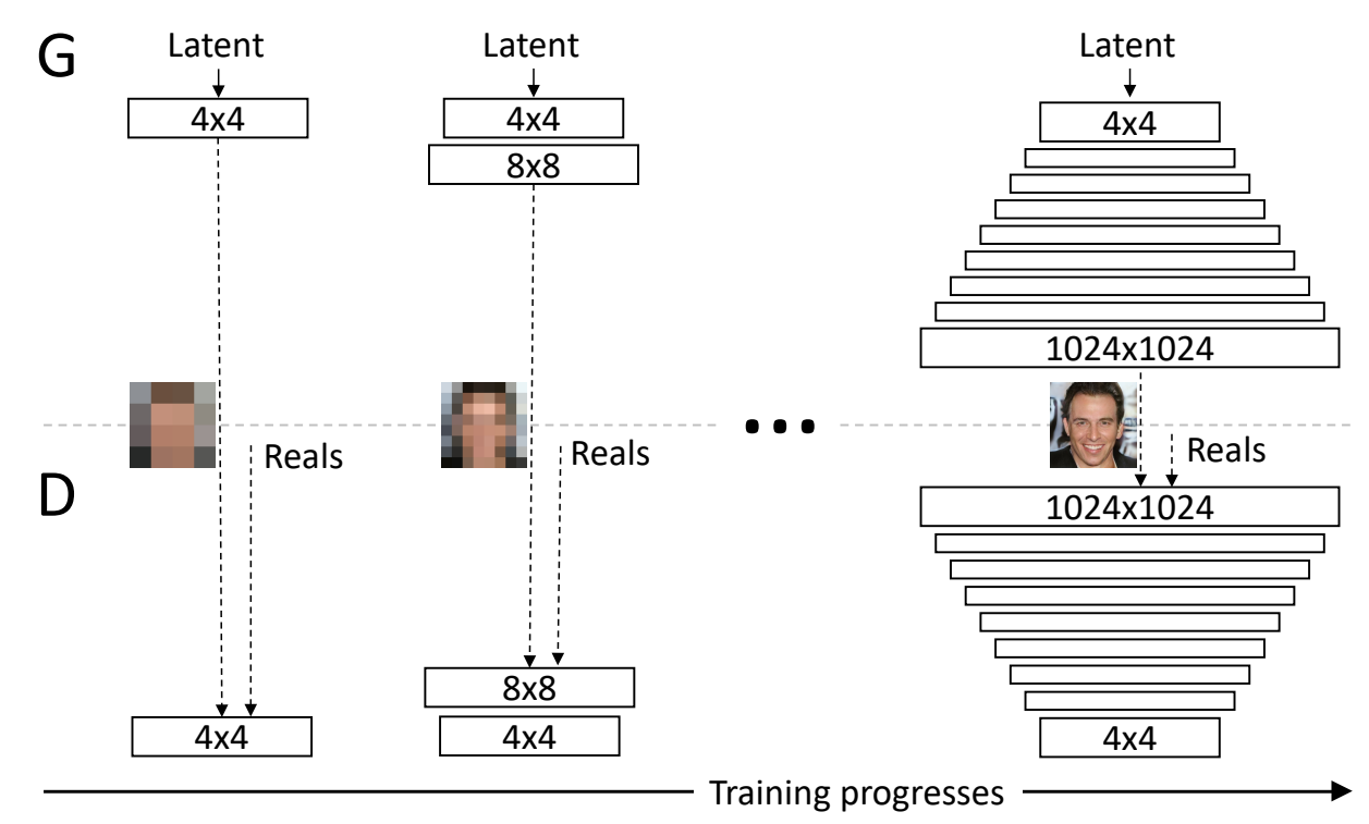
The primary ideology of the ProGAN network is to build upon layers, starting from the lowest to the highest. In the following research paper, the authors have described the methodology upon which both the generators and discriminators learn progressively. As represented in the image above, we start with a 4 x 4 low-resolution image, to which we then start to add additional fine-tuning and higher parameter variables to achieve more effective results. The network first learns and understands the working of a 4 x 4 image. Once that is completed, we proceed to teach it 8 x 8 images, 16 x 16 resolutions, and so on. The highest resolution used in the above example is 1024 x 1024.

This method of progressive training allows the model to achieve unprecedented results with overall higher stability during the entire training process. We have understood that one of the primary ideas for this revolutionary network is to make use of progressively growing techniques. We also previously noted that it doesn't dwell too much into loss functions for these networks like other architectures. A default Wasserstein loss was used in this experimentation, but also other similar loss functions like the least-squares loss can also be utilized. The viewers can learn more about this loss from one of my previous articles on Wasserstein Generative Adversarial Networks (WGAN) from this link.

Apart from the concept of progressive growing networks, the paper also introduces some other significant topics, namely minibatch standard deviation, fading in new layers, pixel normalization, and equalized learning rate. We will explore and understand each of these concepts in further detail in this section before we proceed to their implementation.

The minibatch standard deviation encourages the generative network to create more variations in the generated images as only mini-batches are considered. Since only mini-batches are considered, the discriminator adapts to distinguishing the images as real or fake easier, forcing the generator to generate images with more variety. This simple technique fixes one of the major issues of generative networks, which often have less variation in their generated images in comparison to their respective training data.

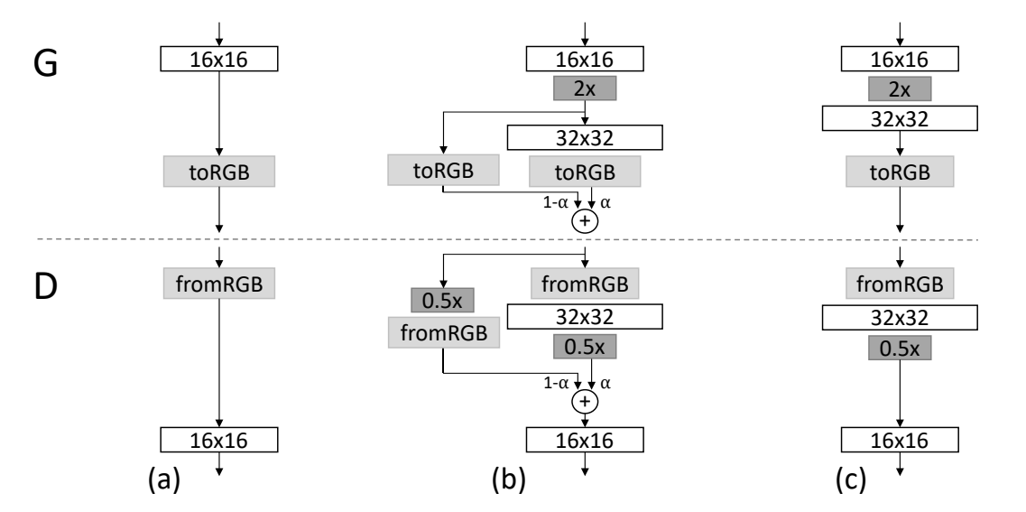
The other significant concept discussed in the research paper is the introduction of fading in new layers. When the transition happens from one phase to another, i.e., switching from the lower resolution to the next higher resolution, the new layers are smoothly faded in. This prevents the previous layers from a sudden "shock" upon the addition of this new layer. The parameter $\alpha$ is used for controlling the fading. This parameter is linearly interpolated over multiple training iterations. As shown in the above image, the final formulation can be written as follows:

$$ (1-\alpha) \times Upsampled \, Layer + (\alpha) \times Output \, Layer $$

The final two concepts we will briefly touch upon in this section are equalized learning rate and pixel normalization. With equalized learning rates, we can scale the weights of each layer accordingly. The formulation is similar to the Kaiming Initialization or He Initialization. But instead of using it as a single initializer, the equalized learning rate uses this in each forward pass. Finally, pixel normalization is used instead of batch normalization as it was noticed that the issue of internal covariate shift is not that prominent in GANs. Pixel Normalization normalizes the feature vector in each pixel to unit length. With the understanding of these basic concepts, we can proceed to construct the ProGAN network architecture for generating facial images.

Constructing ProGAN architectural network from scratch:

In this section, we will cover most of the necessary elements required for constructing the Progressive Growing Generative Adversarial Networks from scratch. We will work on generating facial images with these network architectures. The primary requirements for completing this coding build are a decent GPU for training (or the Paperspace Gradient Platform) and some basic knowledge of the TensorFlow and Keras deep learning frameworks. If you are not familiar with these two libraries, I would recommend checking out this link for TensorFlow and the following link for Keras. Let us get started by importing the necessary libraries.

Importing the essential libraries:

In the first step, we will import all the essential libraries that will be required for computing the ProGAN network effectively. We will import the TensorFlow and Keras deep learning frameworks for building the optimal discriminator and generator networks. The NumPy library will be utilized for most of the mathematical operations that need to be performed. We will also make use of some computer vision libraries to handle images accordingly. Additionally, the mtcnn library can be installed with a simple pip install command. Below is the code snippet representing all the required libraries for this project.

from math import sqrt
from numpy import load, asarray, zeros, ones, savez_compressed
from numpy.random import randn, randint
from skimage.transform import resize
from tensorflow.keras.optimizers import Adam
from tensorflow.keras.models import Sequential, Model
from tensorflow.keras.layers import Input, Dense, Flatten, Reshape, Conv2D
from tensorflow.keras.layers import UpSampling2D, AveragePooling2D, LeakyReLU, Layer, Add
from keras.constraints import max_norm
from keras.initializers import RandomNormal
import mtcnn
from mtcnn.mtcnn import MTCNN
from keras import backend
from matplotlib import pyplot
import cv2
import os
from os import listdir
from PIL import Image
import cv2

Pre-processing the data:

The dataset for this project can be downloaded from the following website. The CelebFaces Attributes (CelebA) Dataset is one of the more popular datasets for tasks related to facial detection and recognition. In this article, we will mainly use this data for the generation of new unique faces with the help of our ProGAN network. Some of the basic functions that we will define in the next code block will help us to handle the project in a more suitable manner. Firstly, we will define a function to load the image, convert it into an RGB image, and store it in the form of a numpy array.

In the next couple of functions, we will make use of the pre-trained Multi-Task Cascaded Convolutional Neural Network (MTCNN), which is considered to be a state-of-the-art accuracy deep learning model for face detection. The primary purpose of using this model is to ensure that we only consider the faces that are available in this celeb dataset while ignoring some of the unnecessary background features. Hence, before resizing the image to the required size, we will perform facial detection and extraction using this mtcnn library that we previously installed on the local system.

# Loading the image file
def load_image(filename):
    image = Image.open(filename)
    image = image.convert('RGB')
    pixels = asarray(image)
    return pixels
    
# extract the face from a loaded image and resize
def extract_face(model, pixels, required_size=(128, 128)):
    # detect face in the image
    faces = model.detect_faces(pixels)
    if len(faces) == 0:
        return None
    
    # extract details of the face
    x1, y1, width, height = faces[0]['box']
    x1, y1 = abs(x1), abs(y1)
    
    x2, y2 = x1 + width, y1 + height
    face_pixels = pixels[y1:y2, x1:x2]
    image = Image.fromarray(face_pixels)
    image = image.resize(required_size)
    face_array = asarray(image)
    
    return face_array
    
# load images and extract faces for all images in a directory
def load_faces(directory, n_faces):
    # prepare model
    model = MTCNN()
    faces = list()
    
    for filename in os.listdir(directory):
        # Computing the retrieval and extraction of faces
        pixels = load_image(directory + filename)
        face = extract_face(model, pixels)
        if face is None:
            continue
        faces.append(face)
        print(len(faces), face.shape)
        if len(faces) >= n_faces:
            break
            
    return asarray(faces)

Depending on your system capabilities, the next step might take some time to fully compute. There is a lot of data available in the dataset. If the readers have more time and computational resources, it is best to extract the entire data and train on the complete CelebA dataset. However, for the purpose of this article, I will utilize only 10000 images for my personal training. Using the below code snippet, we can extract the data and save it in a .npz compressed format for future use.

# load and extract all faces
directory = 'img_align_celeba/img_align_celeba/'
all_faces = load_faces(directory, 10000)
print('Loaded: ', all_faces.shape)

# save in compressed format
savez_compressed('img_align_celeba_128.npz', all_faces)

The saved data can be loaded as shown in the below code snippet.

# load the prepared dataset
from numpy import load
data = load('img_align_celeba_128.npz')
faces = data['arr_0']
print('Loaded: ', faces.shape)

Building the essential functions:

In this section, we will focus on building all the functions that we previously discussed while understanding how ProGANs work. We will first construct the pixel normalization function that will allow us to normalize the feature vector in each pixel to unit length. The below code snippet can be used for computing the pixel normalization accordingly.

# pixel-wise feature vector normalization layer
class PixelNormalization(Layer):
    # initialize the layer
    def __init__(self, **kwargs):
        super(PixelNormalization, self).__init__(**kwargs)
 
    # perform the operation
    def call(self, inputs):
        # computing pixel values
        values = inputs**2.0
        mean_values = backend.mean(values, axis=-1, keepdims=True)
        mean_values += 1.0e-8
        l2 = backend.sqrt(mean_values)
        normalized = inputs / l2
        return normalized
 
    # define the output shape of the layer
    def compute_output_shape(self, input_shape):
        return input_shape

In the next important method that we previously discussed, we will ensure that the model trains on a minibatch standard deviation. The mini-batch functionality is utilized only in the output layer of the discriminator network. We make use of the minibatch standard deviation for ensuring that the model considers smaller batches allowing the variety of images generated to be more unique. Below is the code snippet for computing the minibatch standard deviation.

# mini-batch standard deviation layer
class MinibatchStdev(Layer):
    # initialize the layer
    def __init__(self, **kwargs):
        super(MinibatchStdev, self).__init__(**kwargs)
 
    # perform the operation
    def call(self, inputs):
        mean = backend.mean(inputs, axis=0, keepdims=True)
        squ_diffs = backend.square(inputs - mean)
        mean_sq_diff = backend.mean(squ_diffs, axis=0, keepdims=True)
        mean_sq_diff += 1e-8
        stdev = backend.sqrt(mean_sq_diff)
        
        mean_pix = backend.mean(stdev, keepdims=True)
        shape = backend.shape(inputs)
        output = backend.tile(mean_pix, (shape[0], shape[1], shape[2], 1))
        
        combined = backend.concatenate([inputs, output], axis=-1)
        return combined
 
    # define the output shape of the layer
    def compute_output_shape(self, input_shape):
        input_shape = list(input_shape)
        input_shape[-1] += 1
        return tuple(input_shape)

In the next step, we will compute the weighted sum and define the Wasserstein loss function. The weighted sum class will be utilized for the fading in the layers smoothly, as discussed previously. We will compute the output with the $\alpha$ values, as we formulated in the previous section. Below is the code block for the following actions.

# weighted sum output
class WeightedSum(Add):
    # init with default value
    def __init__(self, alpha=0.0, **kwargs):
        super(WeightedSum, self).__init__(**kwargs)
        self.alpha = backend.variable(alpha, name='ws_alpha')
 
    # output a weighted sum of inputs
    def _merge_function(self, inputs):
        # only supports a weighted sum of two inputs
        assert (len(inputs) == 2)
        # ((1-a) * input1) + (a * input2)
        output = ((1.0 - self.alpha) * inputs[0]) + (self.alpha * inputs[1])
        return output

# calculate wasserstein loss
def wasserstein_loss(y_true, y_pred):
    return backend.mean(y_true * y_pred)

Finally, we will define some of the basic functions that will be required for creating the ProGAN network architecture for the image synthesis project. We will define functions to generate real and fake samples for the generator and discriminator networks. We will then update the fade-in values and scale the dataset accordingly. All these steps are defined in their respective functions available from the code snippet defined below.

# load dataset
def load_real_samples(filename):
    data = load(filename)
    X = data['arr_0']
    X = X.astype('float32')
    X = (X - 127.5) / 127.5
    return X
 
# select real samples
def generate_real_samples(dataset, n_samples):
    ix = randint(0, dataset.shape[0], n_samples)
    X = dataset[ix]
    y = ones((n_samples, 1))
    return X, y
 
# generate points in latent space as input for the generator
def generate_latent_points(latent_dim, n_samples):
    x_input = randn(latent_dim * n_samples)
    x_input = x_input.reshape(n_samples, latent_dim)
    return x_input
 
# use the generator to generate n fake examples, with class labels
def generate_fake_samples(generator, latent_dim, n_samples):
    x_input = generate_latent_points(latent_dim, n_samples)
    X = generator.predict(x_input)
    y = -ones((n_samples, 1))
    return X, y
 
# update the alpha value on each instance of WeightedSum
def update_fadein(models, step, n_steps):
    alpha = step / float(n_steps - 1)
    for model in models:
        for layer in model.layers:
            if isinstance(layer, WeightedSum):
                backend.set_value(layer.alpha, alpha)
                
# scale images to preferred size
def scale_dataset(images, new_shape):
    images_list = list()
    for image in images:
        new_image = resize(image, new_shape, 0)
        images_list.append(new_image)
    return asarray(images_list)

Creating the generator network:

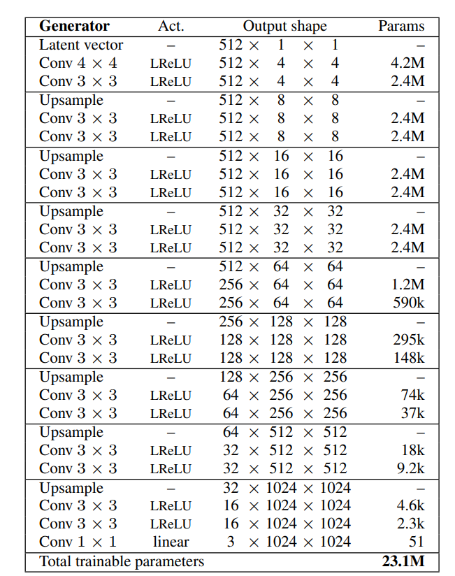
The generator architecture includes a latent vector space where we can initialize our initial parameters to generate the desired image. Once we define the latent vector space, we will obtain a 4 x 4 dimensionality that will allow us to deal with the initial input image. We will then continue to add upsampling and convolutional layers along with pixel normalization layers for a few blocks with the leaky ReLU activation function. Finally, we will add a 1 x 1 convolution to map the RGB image.

The generator developed will utilize most of the features from the research paper apart from some minor exceptions. Instead of using 512 or increasing filters, we will make use of 128 filters as we are constructing the architecture with smaller image sizes. Instead of the equalized learning rate, we will make use of Gaussian random numbers and the max norm weight constraint. We will first define a generator block and then develop the entire generator model network. Below is the code snippet for the generator block.

# adding a generator block
def add_generator_block(old_model):
    init = RandomNormal(stddev=0.02)
    const = max_norm(1.0)
    block_end = old_model.layers[-2].output
    
    # upsample, and define new block
    upsampling = UpSampling2D()(block_end)
    g = Conv2D(128, (3,3), padding='same', kernel_initializer=init, kernel_constraint=const)(upsampling)
    g = PixelNormalization()(g)
    g = LeakyReLU(alpha=0.2)(g)
    g = Conv2D(128, (3,3), padding='same', kernel_initializer=init, kernel_constraint=const)(g)
    g = PixelNormalization()(g)
    g = LeakyReLU(alpha=0.2)(g)
    
    out_image = Conv2D(3, (1,1), padding='same', kernel_initializer=init, kernel_constraint=const)(g)
    model1 = Model(old_model.input, out_image)
    out_old = old_model.layers[-1]
    out_image2 = out_old(upsampling)
    
    merged = WeightedSum()([out_image2, out_image])
    model2 = Model(old_model.input, merged)
    return [model1, model2]

Below is the code snippet for completing the generator architecture for each successive layer.

# define generator models
def define_generator(latent_dim, n_blocks, in_dim=4):
    init = RandomNormal(stddev=0.02)
    const = max_norm(1.0)
    model_list = list()
    in_latent = Input(shape=(latent_dim,))
    g  = Dense(128 * in_dim * in_dim, kernel_initializer=init, kernel_constraint=const)(in_latent)
    g = Reshape((in_dim, in_dim, 128))(g)
    
    # conv 4x4, input block
    g = Conv2D(128, (3,3), padding='same', kernel_initializer=init, kernel_constraint=const)(g)
    g = PixelNormalization()(g)
    g = LeakyReLU(alpha=0.2)(g)
    
    # conv 3x3
    g = Conv2D(128, (3,3), padding='same', kernel_initializer=init, kernel_constraint=const)(g)
    g = PixelNormalization()(g)
    g = LeakyReLU(alpha=0.2)(g)
    
    # conv 1x1, output block
    out_image = Conv2D(3, (1,1), padding='same', kernel_initializer=init, kernel_constraint=const)(g)
    model = Model(in_latent, out_image)
    model_list.append([model, model])
    
    for i in range(1, n_blocks):
        old_model = model_list[i - 1][0]
        models = add_generator_block(old_model)
        model_list.append(models)
        
    return model_list

Creating the discriminator network:

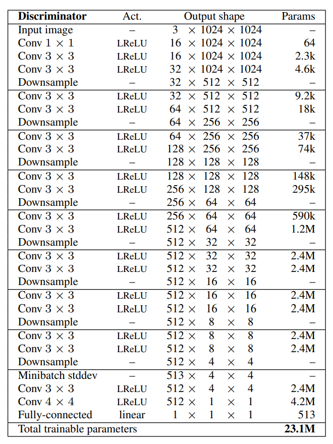
For the discriminator architecture, we will somewhat reverse engineer the way the generator network was built. We will start with an RGB image and pass it through a bunch of convolutional layers with downsampling. A bunch of blocks will repeat this pattern, but towards the end, at the output block, we will add a minibatch standard deviation layer concatenated with the previous outputs. Finally, after two additional convolutional layers, we will make the discriminator output a single output, which determines if the generated image is fake or real. Below is the code snippet for adding a discriminator block.

# adding a discriminator block
def add_discriminator_block(old_model, n_input_layers=3):
    init = RandomNormal(stddev=0.02)
    const = max_norm(1.0)
    in_shape = list(old_model.input.shape)
    
    # define new input shape as double the size
    input_shape = (in_shape[-2]*2, in_shape[-2]*2, in_shape[-1])
    in_image = Input(shape=input_shape)
    
    # define new input processing layer
    d = Conv2D(128, (1,1), padding='same', kernel_initializer=init, kernel_constraint=const)(in_image)
    d = LeakyReLU(alpha=0.2)(d)
    
    # define new block
    d = Conv2D(128, (3,3), padding='same', kernel_initializer=init, kernel_constraint=const)(d)
    d = LeakyReLU(alpha=0.2)(d)
    d = Conv2D(128, (3,3), padding='same', kernel_initializer=init, kernel_constraint=const)(d)
    d = LeakyReLU(alpha=0.2)(d)
    d = AveragePooling2D()(d)
    block_new = d
    
    # skip the input, 1x1 and activation for the old model
    for i in range(n_input_layers, len(old_model.layers)):
        d = old_model.layers[i](d)
    model1 = Model(in_image, d)
    
    model1.compile(loss=wasserstein_loss, optimizer=Adam(lr=0.001, beta_1=0, beta_2=0.99, epsilon=10e-8))
    
    downsample = AveragePooling2D()(in_image)
    
    block_old = old_model.layers[1](downsample)
    block_old = old_model.layers[2](block_old)
    d = WeightedSum()([block_old, block_new])
    
    for i in range(n_input_layers, len(old_model.layers)):
        d = old_model.layers[i](d)
        
    model2 = Model(in_image, d)
    
    model2.compile(loss=wasserstein_loss, optimizer=Adam(lr=0.001, beta_1=0, beta_2=0.99, epsilon=10e-8))
    return [model1, model2]

Below is the code snippet for completing the discriminator architecture for each successive layer.

# define the discriminator models for each image resolution
def define_discriminator(n_blocks, input_shape=(4,4,3)):
    init = RandomNormal(stddev=0.02)
    const = max_norm(1.0)
    model_list = list()
    in_image = Input(shape=input_shape)
    
    d = Conv2D(128, (1,1), padding='same', kernel_initializer=init, kernel_constraint=const)(in_image)
    d = LeakyReLU(alpha=0.2)(d)
    d = MinibatchStdev()(d)
    
    d = Conv2D(128, (3,3), padding='same', kernel_initializer=init, kernel_constraint=const)(d)
    d = LeakyReLU(alpha=0.2)(d)
    d = Conv2D(128, (4,4), padding='same', kernel_initializer=init, kernel_constraint=const)(d)
    d = LeakyReLU(alpha=0.2)(d)
    
    d = Flatten()(d)
    out_class = Dense(1)(d)
    
    model = Model(in_image, out_class)
    model.compile(loss=wasserstein_loss, optimizer=Adam(lr=0.001, beta_1=0, beta_2=0.99, epsilon=10e-8))
    model_list.append([model, model])
    
    for i in range(1, n_blocks):
        old_model = model_list[i - 1][0]
        models = add_discriminator_block(old_model)
        model_list.append(models)
        
    return model_list

Developing the ProGAN model architecture:

Once we have finished defining the individual generator and discriminator networks, we will create an overall composite model that combines both of them to create the ProGAN model architecture. Once we combine the generator models, we can compile them and train them accordingly. Let us define the function to create the composite ProGAN network.

# define composite models for training generators via discriminators

def define_composite(discriminators, generators):
    model_list = list()
    # create composite models
    for i in range(len(discriminators)):
        g_models, d_models = generators[i], discriminators[i]
        # straight-through model
        d_models[0].trainable = False
        model1 = Sequential()
        model1.add(g_models[0])
        model1.add(d_models[0])
        model1.compile(loss=wasserstein_loss, optimizer=Adam(lr=0.001, beta_1=0, beta_2=0.99, epsilon=10e-8))
        # fade-in model
        d_models[1].trainable = False
        model2 = Sequential()
        model2.add(g_models[1])
        model2.add(d_models[1])
        model2.compile(loss=wasserstein_loss, optimizer=Adam(lr=0.001, beta_1=0, beta_2=0.99, epsilon=10e-8))
        # store
        model_list.append([model1, model2])
    return model_list

Finally, once we have created the overall composite model, we can begin the training process. Most of the steps involved in training the network are similar to how we have previously trained GANs. However, the fade-in layers and the progressive update of the progressively growing GAN are also introduced during the training process. Below is the code block for creating the training epochs.

# train a generator and discriminator
def train_epochs(g_model, d_model, gan_model, dataset, n_epochs, n_batch, fadein=False):
    bat_per_epo = int(dataset.shape[0] / n_batch)
    n_steps = bat_per_epo * n_epochs
    half_batch = int(n_batch / 2)
    
    for i in range(n_steps):
        # update alpha for all WeightedSum layers when fading in new blocks
        if fadein:
            update_fadein([g_model, d_model, gan_model], i, n_steps)
        # prepare real and fake samples
        X_real, y_real = generate_real_samples(dataset, half_batch)
        X_fake, y_fake = generate_fake_samples(g_model, latent_dim, half_batch)
        
        # update discriminator model
        d_loss1 = d_model.train_on_batch(X_real, y_real)
        d_loss2 = d_model.train_on_batch(X_fake, y_fake)
        
        # update the generator via the discriminator's error
        z_input = generate_latent_points(latent_dim, n_batch)
        y_real2 = ones((n_batch, 1))
        g_loss = gan_model.train_on_batch(z_input, y_real2)
        
        # summarize loss on this batch
        print('>%d, d1=%.3f, d2=%.3f g=%.3f' % (i+1, d_loss1, d_loss2, g_loss))
        
# train the generator and discriminator
def train(g_models, d_models, gan_models, dataset, latent_dim, e_norm, e_fadein, n_batch):
    g_normal, d_normal, gan_normal = g_models[0][0], d_models[0][0], gan_models[0][0]
    gen_shape = g_normal.output_shape
    scaled_data = scale_dataset(dataset, gen_shape[1:])
    print('Scaled Data', scaled_data.shape)

    # train normal or straight-through models
    train_epochs(g_normal, d_normal, gan_normal, scaled_data, e_norm[0], n_batch[0])
    summarize_performance('tuned', g_normal, latent_dim)
    
    # process each level of growth
    for i in range(1, len(g_models)):
        # retrieve models for this level of growth
        [g_normal, g_fadein] = g_models[i]
        [d_normal, d_fadein] = d_models[i]
        [gan_normal, gan_fadein] = gan_models[i]
        
        # scale dataset to appropriate size
        gen_shape = g_normal.output_shape
        scaled_data = scale_dataset(dataset, gen_shape[1:])
        print('Scaled Data', scaled_data.shape)
        
        # train fade-in models for next level of growth
        train_epochs(g_fadein, d_fadein, gan_fadein, scaled_data, e_fadein[i], n_batch[i], True)
        summarize_performance('faded', g_fadein, latent_dim)
        
        # train normal or straight-through models
        train_epochs(g_normal, d_normal, gan_normal, scaled_data, e_norm[i], n_batch[i])
        summarize_performance('tuned', g_normal, latent_dim)

During the training, we will also define a custom function that will help us to evaluate our results accordingly. We can summarize our performance as well as plot some of the figures generated from each iteration to see how good our improvement of the results is. Below is the code snippet for summarizing our overall model performance.

# generate samples and save as a plot and save the model
def summarize_performance(status, g_model, latent_dim, n_samples=25):
    gen_shape = g_model.output_shape
    name = '%03dx%03d-%s' % (gen_shape[1], gen_shape[2], status)
    
    X, _ = generate_fake_samples(g_model, latent_dim, n_samples)
    X = (X - X.min()) / (X.max() - X.min())
    
    square = int(sqrt(n_samples))
    for i in range(n_samples):
        pyplot.subplot(square, square, 1 + i)
        pyplot.axis('off')
        pyplot.imshow(X[i])
        
    # save plot to file
    filename1 = 'plot_%s.png' % (name)
    pyplot.savefig(filename1)
    pyplot.close()
    
    filename2 = 'model_%s.h5' % (name)
    g_model.save(filename2)
    print('>Saved: %s and %s' % (filename1, filename2))

Finally, once all the necessary functions are defined accordingly, we can begin the training process. To increase stability, we will use larger batch sizes and lesser epochs for small image sizes while reducing the batch size and increasing the number of epochs towards the larger scaling of images. The code snippet for training the ProGAN network for image synthesis is shown below.

# number of growth phases where 6 blocks == [4, 8, 16, 32, 64, 128]
n_blocks = 6
latent_dim = 100

d_models = define_discriminator(n_blocks)
g_models = define_generator(latent_dim, n_blocks)
gan_models = define_composite(d_models, g_models)

dataset = load_real_samples('img_align_celeba_128.npz')
print('Loaded', dataset.shape)

n_batch = [16, 16, 16, 8, 4, 4]
n_epochs = [5, 8, 8, 10, 10, 10]

train(g_models, d_models, gan_models, dataset, latent_dim, n_epochs, n_epochs, n_batch)

Results and further discussion:

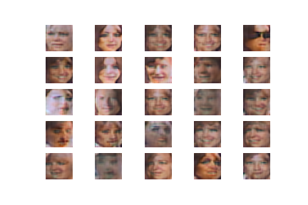
>12500, d1=1756536064.000, d2=8450036736.000 g=-378913792.000
Saved: plot_032x032-faded.png and model_032x032-faded.h5

The result I obtained after just 32 x 32 upsampling after multiple epochs of training is shown in the figure below.

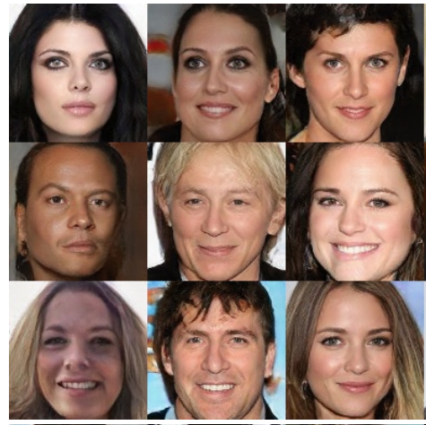
Ideally, if you had more time, images, and computational resources to train, we would have been able to obtain results similar to the image shown below.

The majority of the code is considered from the machine learning repository website, which I would highly recommend checking out from the following link. There are several improvements and additions that can be made to the following project. We can improve the dataset by using higher image qualities, increasing the training iterations and overall computational capabilities. Another idea is to merge the ProGAN network with the SRGAN architecture to create unique combination possibilities. I would suggest the interested readers experiment with the numerous possible outcomes.

Conclusion:

Everything that living things learn is in little (or baby) steps, either by adapting from previous mistakes or learning from scratch while slowly developing each individual aspect of any particular concept, idea, or imagination. Instead of directly creating large sentences, we are first taught alphabets and letters, small words, and so on till we are able to construct longer sentences. Similarly, the ProGAN network uses a similarly intuitive approach where the model starts learning from the lowest pixel resolution. It then gradually learns in an increasing pattern of higher resolutions to achieve a high-quality result at the end of the spectrum.

In this article, we covered most of the topics required to gain a basic intuitive understanding of the ProGAN networks for high-quality image generation. We started with a basic introduction of the ProGAN networks and then proceeded to understand most of the unique aspects that were introduced in its research paper by its authors to accomplish unprecedented results. Finally, we used the obtained knowledge to construct a ProGAN network from scratch for the generation of facial images using the Celeb-A dataset. While the training was done for a limited resolution, the readers can carry out further experiments all the way up to higher qualities of resolution. There is an endless possibility of advancements that can be made to these generative networks.

In the upcoming articles, we will cover more variations of Generative Adversarial Networks, such as the StyleGAN architecture and so much more. We will also gain a conceptual understanding of variational autoencoders as well as work on more signal processing projects. Until then, keep experimenting and coding more unique deep learning and AI projects!