Network in Network: Utility of 1 x 1 Convolution Layers

Down-sampling is a beneficial process in convolutional neural networks as it helps to progressively manage the amount of pixels/data present in the network, thereby helping to manage computation time during training. As we know by now, feature maps in a convolution layer are 4 dimensional, (batch size, channels, height, width) with pooling allowing us to down-sample along the height and width dimensions. It is also possible to down-sample along the channel dimension through a process called 1 x 1 convolution.

In this article, we will be taking a look at 1 x 1 convolution not only as a down-sampling tool but across its several usages in convolutional neural networks.

#  article dependencies
import torch
import torch.nn as nn
import torch.nn.functional as F
import time

The Concept of 1 x 1 Convolution

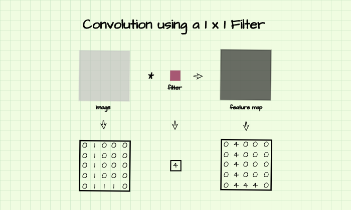
First introduced in the paper 'Network in Network' (Min Lin et al, 2013), 1 x 1 convolution is a process of performing a convolution operation using a filter with just one row and one column. Essentially, it is the process of performing convolution using a scaler value (a single number) rather than a matrix as is typical to convolution layers, and as such it basically does not extract features, per say.

In more technical terms, 1 x 1 convolution can be said to be a pixel-wise weighting of feature maps since each pixel is multiplied by a single number without regard for neighboring pixels. In the image below, 1 x 1 convolution is performed on the matrix using the given filter. The resulting feature map is a representation of the original matrix with pixel values 4 times the original, therefore the original image is said to have been weighted by 4 using the filter.

1 x 1 Convolution & Dimensionality Reduction

As convolutional neural networks become deeper, the number of channels/feature maps in their layers progressively increase in number. In fact, It's not unusual to have as many as 512 feature maps in an intermediate convolution layer.

What can be done to to keep the number of feature maps in check? Let's assume one would like to build a deeper network, but there are already 512 feature maps in an intermediate layer and this is deemed excessive, one could easily apply 1 x 1 convolution to reduce the number of feature maps to, say 32, and then continue to add more convolution layers. For instance, if there are (512, 12, 12) (512 representations, each of size 12 pixels by 12 pixels) feature maps in a convolution layer we could simply apply (32, 512, 1, 1) (32 1 x 1 convolution filters, each with 512 channels) filters to reduce the number of feature maps to 32, thereby producing (32, 12, 12) feature maps as seen below.

#  output from an intermediate layer
intermediate_output = torch.ones((512, 12, 12))

#  1x1 convolution layer
conv_1x1 = nn.Conv2d(512, 32, 1)

#  producing a downsampled representation 
downsampled = conv_1x1(intermediate_output)
downsampled.shape

#  output
>>>> torch.Size([32, 12, 12])

Theoretically, the above mentioned process could also be done using a regular convolution filter, but the difference will be that features will not be summarized across channels; rather, new features will be learnt. Since 1 x 1 convolution is simply a weighting of individual pixels, without considering neighboring pixels, followed by summation across channels, it can be said to be a kind of channel-wise pooling. Hence, the 32 feature maps produced will be 'summaries' of all 512 feature maps present in the layer.

Lastly, down-sampling using a regular convolution filter is more computationally expensive. For instance, suppose one would like to down-sample from 512 to 32 feature maps using a (3, 3) filter, that would result in 147,488 parameters (512*32*3*3 weights + 32 biases) as opposed to 16,416 parameters (512*32*1*1 weights + 32 biases) when done with a (1, 1) filter.

#  1x1 convolution layer
conv_1x1 = nn.Conv2d(512, 32, 1)

#  3x3 convolution layer
conv_3x3 = nn.Conv2d(512, 32, 3, padding=1)

#  deriving parameters in the network
parameters_1x1 = list(conv_1x1.parameters())
parameters_3x3 = list(conv_3x3.parameters())

#  deriving total number of parameters in the (1, 1) layer
number_of_parameters_1x1 = sum(x.numel() for x in parameters_1x1)
#  output
>>>> 16,416

#  deriving total number of parameters in the (3, 3) layer
number_of_parameters_3x3 = sum(x.numel() for x in parameters_3x3)
#  output
>>>> 147,488

The disparity in parameters also translates into speed of computation with down-sampling using (1, 1) filters being approximately 23 times faster than when the same process is done with a (3, 3) filter.

#  start time
start = time.time()

#  producing downsampled representation 
downsampled = conv_1x1(intermediate_output)

#  stop time
stop = time.time()

print(round(stop-start, 5))
#  output
>>>> 0.00056

#  start time
start = time.time()

#  producing downsampled representation 
downsampled = conv_3x3(intermediate_output)

#  stop time
stop = time.time()

print(round(stop-start, 5))
#  output
>>>> 0.01297

Additional Non-Linearity with 1 x 1 Convolutions

Since ReLU activation typically follows 1 x 1 convolution layers, we could essentially include them (1 x 1 convolution layers) without performing dimensionality reduction just for the extra ReLU non-linearity that comes along with them. For instance, the feature map of size (512, 12, 12) from the previous section could be convolved using (512, 512, 1, 1) (512 1 x 1 convolution filters all with 512 channels each) filters to again produce (512, 12, 12) feature maps all just to take advantage of the ReLU non-linearity that follows.

To better illustrate, consider the sample ConvNet in the code block below, layer 3 is a 1 x 1 convolution layer which returns the same number of feature maps as the (3, 3) convolution in layer 2. The 1 x 1 convolution layer in this context is not redundant as it is accompanied by a ReLU activation function which would not have been present in the network. This is beneficial because the additional non-linearities will further force the network to learn a more complex mapping of inputs to outputs thereby enabling the network to generalize better.

class ConvNet(nn.Module):
  def __init__(self):
    super().__init__()
    self.network = nn.Sequential(
        #  layer 1
        nn.Conv2d(1, 3, 3, padding=1),
        nn.MaxPool2d(2),
        nn.ReLU(),
        #  layer 2
        nn.Conv2d(3, 8, 3, padding=1),
        nn.MaxPool2d(2),
        nn.ReLU(),
        #  layer 3
        nn.Conv2d(8, 8, 1),
        nn.ReLU() #  additional non-linearity
    )

  def forward(self, x):
    input = x.view(-1, 1, 28, 28)
    output = self.network(input)
    return output

Replacing Linear Layers Using 1 x 1 Convolution

Imagine building a convolutional neural network architecture for a 10 class multi-class classification task. In a classical convolutional neural network architecture, the convolution layers serve as feature extractors while the linear layers vectorize the feature maps in stages up until a 10 element vector representation holding each class' confidence scores is returned. The problem with linear layers is they easily overfit during training requiring dropout regularization as a mitigative measure.

class ConvNet(nn.Module):
  def __init__(self):
    super().__init__()
    self.conv1 = nn.Conv2d(1, 3, 3, padding=1)
    self.pool1 = nn.MaxPool2d(2)
    self.conv2 = nn.Conv2d(3, 64, 3, padding=1)
    self.pool2 = nn.MaxPool2d(2)
    self.linear1 = nn.Linear(3136, 100)
    self.linear2 = nn.Linear(100, 10)


  def forward(self, x):
    input = x.view(-1, 1, 28, 28)

    #-----------
    # LAYER 1
    #-----------
    output_1 = self.conv1(input)
    output_1 = self.pool1(output_1)
    output_1 = F.relu(output_1)

    #-----------
    # LAYER 2
    #-----------
    output_2 = self.conv2(output_1)
    output_2 = self.pool2(output_2)
    output_2 = F.relu(output_2)

    #  flattening feature maps
    output_2 = output_2.view(-1, 7*7*64)

    #-----------
    # LAYER 3
    #-----------
    output_3 = self.linear1(output_2)
    output_3 = F.relu(output_3)

    #--------------
    # OUTPUT LAYER
    #--------------
    output_4 = self.linear2(output_3)
    
    return torch.sigmoid(output_4)

Incorporating 1 x 1 convolutions, one could get rid of the linear layers entirely by down-sampling the number of feature maps until they are of the same as the number of classes in the task at hand (10 in this case). Next, the mean value of all pixels in each feature map is returned to produce a 10 element vector holding confidence scores for each class (this process is called global average pooling, more on this in a coming article).

class ConvNet(nn.Module):
  def __init__(self):
    super().__init__()
    self.conv1 = nn.Conv2d(1, 3, 3, padding=1)
    self.pool1 = nn.MaxPool2d(2)
    self.conv2 = nn.Conv2d(3, 64, 3, padding=1)
    self.pool2 = nn.MaxPool2d(2)
    self.conv3 = nn.Conv2d(64, 32, 1) # 1 x 1 downsampling from 64 channels to 32 channels
    self.conv4 = nn.Conv2d(32, 10, 1) # 1 x 1 downsampling from 32 channels to 10 channels
    self.pool4 = nn.AvgPool2d(7) # deriving average pixel values per channel


  def forward(self, x):
    input = x.view(-1, 1, 28, 28)

    #-----------
    # LAYER 1
    #-----------
    output_1 = self.conv1(input)
    output_1 = self.pool1(output_1)
    output_1 = F.relu(output_1)

    #-----------
    # LAYER 2
    #-----------
    output_2 = self.conv2(output_1)
    output_2 = self.pool2(output_2)
    output_2 = F.relu(output_2)

    #-----------
    # LAYER 3
    #-----------
    output_3 = self.conv3(output_2)
    output_3 = F.relu(output_3)

    #--------------
    # OUTPUT LAYER
    #--------------
    output_4 = self.conv4(output_3)
    output_4 = self.pool4(output_4)
    output_4 = output_4.view(-1, 10)
    
    return torch.sigmoid(output_4)

Final Remarks

In this article, we took a look at 1 x 1 convolution and its various purposes in convolutional neural networks. We looked through the process itself and how it is used as a dimensionality reduction tool, as a source of additional non-linearity and as a means to exclude linear layers in CNN architectures and mitigate the problem of overfitting. This process is a mainstay in several state of the art convolutional neural network architectures and is definitely a great concept to properly grasp and understand.